AlphaFold 2, FourCastNet and CorrDiff are exciting. AI-driven autonomous labs are going to be a big deal [1]. Science codes now use AI and machine learning to make scientific discoveries on the world’s most powerful computers [2].
It’s common practice for scientists to ask questions about the validity, reliability and accuracy of the mathematical and computational methods they use. And many have voiced concerns about the lack of explainability and potential pitfalls of AI models, in particular deep neural networks (DNNs) [3].
The impact of this uncertainty varies highly according to project. Science projects that are able to easily check AI-generated results against ground truth may not be that concerned. High-stakes projects like design of a multimillion dollar spacecraft with high project risks may ask about AI model accuracy with more urgency.
Neural network accuracy
Understanding of the properties of DNNs is still in its infancy, with many as-yet unanswered questions. However, in the last few years some significant results have started to come forth.
A fruitful approach to analyzing DNNs is to see them as function approximators (which, of course, they are). One can study how accurately DNNs approximate a function representing some physical phenomenon in a domain (for example, fluid density or temperature).
The approximation error can be measured in various ways. A particularly strong measure is “sup-norm” or “max-norm” error, which requires that the DNN approximation be accurate at every point of the target function’s domain (“uniform approximation”). Some science problems may have a weaker requirement than this, such as low RMS or 2-norm error. However, it’s not unreasonable to ask about max-norm approximation behaviors of numerical methods [4,5].
An illuminating paper by Ben Adcock and Nick Dexter looks at this problem [6]. They show that standard DNN methods applied even to a simple 1-dimensional problem can result in “glitches”: the DNN as a whole matches the function well but at some points totally misapproximates the target function. For a picture that shows this, see [7].
Other mathematical papers have subsequently shed light on these behaviors. I’ll try to summarize the findings below, though the actual findings are very nuanced, and many details are left out here. The reader is advised to refer to the respective papers for exact details.
The findings address three questions: 1) how many DNN parameters are required to approximate a function well? 2) how much data is required to train to a desired accuracy? and 3) what algorithms are capable of training to the desired accuracy?
How many neural network weights are needed?
How large does the neural network need to be for accurate uniform approximation of functions? If tight max-norm approximation requires an excessively large number of weights, then use of DNNs is not computationally practical.
Some answers to this question have been found—in particular, a result 1 is given in [8, Theorem 4.3; cf. 9, 10]. This result shows that the number of neural network weights required to approximate an arbitrary function to high max-norm accuracy grows exponentially in the dimension of the input to the function.
This dependency on dimension is no small limitation, insofar as this is not the dimension of physical space (e.g., 3-D) but the dimension of the input vector (such as the number of gridcells), which for practical problems can be in the tens [11] or even millions or more.
Sadly, this rules out the practical use of DNN for some purposes. Nonetheless, for many practical applications of deep learning, the approximation behaviors are not nearly so pessimistic as this would indicate (cp. [12]). For example, results are more optimistic:
- if the target function has a strong smoothness property;
- if the function is not arbitrary but is a composition of simpler functions;
- if the training and test data are restricted to a (possibly unknown) lower dimensional manifold in the high dimensional space (this is certainly the case for common image and language modeling tasks);
- if the average case behavior for the desired problem domain is much better than the worst case behavior addressed in the theorem;
- The theorem assumes multilayer perceptron and ReLU activation; other DNN architectures may perform better (though the analysis is based on multidimensional Taylor’s theorem, which one might conjecture applies also to other architectures).
- For many practical applications, very high accuracy is not a requirement.
- For some applications, only low 2-norm error is sufficient, (not low max-norm).
- For the special case of physics informed neural networks (PINNs), stronger results hold.
Thus, not all hope is lost from the standpoint of theory. However, certain problems for which high accuracy is required may not be suitable for DNN approximation.
How much training data is needed?
Assuming your space of neural network candidates is expressive enough to closely represent the target function—how much training data is required to actually find a good approximation?
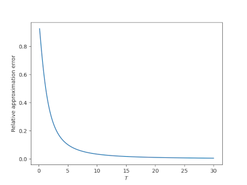
A result 2 is given in [13, Theorem 2.2] showing that the number of training samples required to train to high max-norm accuracy grows, again, exponentially in the dimension of the input to the function.
The authors concede however that “if additional problem information about [the target functions] can be incorporated into the learning problem it may be possible to overcome the barriers shown in this work.” One suspects that some of the caveats given above might also be relevant here. Additionally, if one considers 2-norm error instead of max-norm error, the data requirement grows polynomially rather than exponentially, making the training data requirement much more tractable. Nonetheless, for some problems the amount of data required is so large that attempts to “pin down” the DNN to sufficient accuracy become intractable.
What methods can train to high accuracy?
The amount of training data may be sufficient to specify a suitable neural network. But, will standard methods for finding the weights of such a DNN be effective for solving this difficult nonconvex optimization problem?
A recent paper [14] from Max Tegmark’s group empirically studies DNN training to high accuracy. They find that as the input dimension grows, training to very high accuracy with standard stochastic gradient descent methods becomes difficult or impossible.
They also find second order methods perform much better, though these are more computationally expensive and have some difficulty also when the dimension is higher. Notably, second order methods have been used effectively for DNN training for some science applications [15]. Also, various alternative training approaches have been tried to attempt to stabilize training; see, e.g., [16].
Prospects and conclusions
Application of AI methods to scientific discovery continues to deliver amazing results, in spite of lagging theory. Ilya Sutskever has commented, “Progress in AI is a game of faith. The more faith you have, the more progress you can make” [17].
Theory of deep learning methods is in its infancy. The current findings show some cases for which use of DNN methods may not be fruitful, Continued discoveries in deep learning theory can help better guide how to use the methods effectively and inform where new algorithmic advances are needed.
Footnotes
1 Suppose the function to be approximated takes d inputs and has the smoothness property that all nth partial derivatives are continuous (i.e., is in Cn(Ω) for compact Ω). Also suppose a multilayer perceptron with ReLU activation functions must be able to approximate any such function to max-norm no worse than ε. Then the number of weights required is at least a fixed constant times (1/ε)d/(2n).
2 Let F be the space of all functions that can be approximated exactly by a broad class of ReLU neural networks. Suppose there is a training method that can recover all these functions up to max-norm accuracy bounded by ε. Then the number of training samples required is at least a fixed constant times (1/ε)d.
References
[1] “Integrated Research Infrastructure Architecture Blueprint Activity (Final Report 2023),” https://www.osti.gov/biblio/1984466.
[2] Joubert, Wayne, Bronson Messer, Philip C. Roth, Antigoni Georgiadou, Justin Lietz, Markus Eisenbach, and Junqi Yin. “Learning to Scale the Summit: AI for Science on a Leadership Supercomputer.” In 2022 IEEE International Parallel and Distributed Processing Symposium Workshops (IPDPSW), pp. 1246-1255. IEEE, 2022, https://www.osti.gov/biblio/2076211.
[3] “Reproducibility Workshop: The Reproducibility Crisis in ML‑based Science,” Princeton University, July 28, 2022, https://sites.google.com/princeton.edu/rep-workshop.
[4] Wahlbin, L. B. (1978). Maximum norm error estimates in the finite element method with isoparametric quadratic elements and numerical integration. RAIRO. Analyse numérique, 12(2), 173-202, https://www.esaim-m2an.org/articles/m2an/pdf/1978/02/m2an1978120201731.pdf
[5] Kashiwabara, T., & Kemmochi, T. (2018). Maximum norm error estimates for the finite element approximation of parabolic problems on smooth domains. https://arxiv.org/abs/1805.01336.
[6] Adcock, Ben, and Nick Dexter. “The gap between theory and practice in function approximation with deep neural networks.” SIAM Journal on Mathematics of Data Science 3, no. 2 (2021): 624-655, https://epubs.siam.org/doi/10.1137/20M131309X.
[7] “Figure 5 from The gap between theory and practice in function approximation with deep neural networks | Semantic Scholar,” https://www.semanticscholar.org/paper/The-gap-between-theory-and-practice-in-function-Adcock-Dexter/156bbfc996985f6c65a51bc2f9522da2a1de1f5f/figure/4
[8] Gühring, I., Raslan, M., & Kutyniok, G. (2022). Expressivity of Deep Neural Networks. In P. Grohs & G. Kutyniok (Eds.), Mathematical Aspects of Deep Learning (pp. 149-199). Cambridge: Cambridge University Press. doi:10.1017/9781009025096.004, https://arxiv.org/abs/2007.04759.
[9] D. Yarotsky. Error bounds for approximations with deep ReLU networks. Neural Netw., 94:103–114, 2017, https://arxiv.org/abs/1610.01145
[10] I. Gühring, G. Kutyniok, and P. Petersen. Error bounds for approximations with deep relu neural networks in Ws,p norms. Anal. Appl. (Singap.), pages 1–57, 2019, https://arxiv.org/abs/1902.07896
[11] Matt R. Norman, “The MiniWeather Mini App,” https://github.com/mrnorman/miniWeather
[12] Lin, H.W., Tegmark, M. & Rolnick, D. Why Does Deep and Cheap Learning Work So Well?. J Stat Phys 168, 1223–1247 (2017). https://doi.org/10.1007/s10955-017-1836-5
[13] Berner, J., Grohs, P., & Voigtlaender, F. (2022). Training ReLU networks to high uniform accuracy is intractable. ICLR 2023, https://openreview.net/forum?id=nchvKfvNeX0.
[14] Michaud, E. J., Liu, Z., & Tegmark, M. (2023). Precision machine learning. Entropy, 25(1), 175, https://www.mdpi.com/1099-4300/25/1/175.
[15] Markidis, S. (2021). The old and the new: Can physics-informed deep-learning replace traditional linear solvers?. Frontiers in big Data, 4, 669097, https://www.frontiersin.org/articles/10.3389/fdata.2021.669097/full
[16] Bengio, Y., Lamblin, P., Popovici, D., & Larochelle, H. (2006). Greedy layer-wise training of deep networks. Advances in neural information processing systems, 19, https://papers.nips.cc/paper_files/paper/2006/hash/5da713a690c067105aeb2fae32403405-Abstract.html
[17] “Chat with OpenAI CEO and Co-founder Sam Altman, and Chief Scientist Ilya Sutskever,” https://www.youtube.com/watch?v=mC-0XqTAeMQ&t=250s