Double super factorial

I saw someone point out recently that

10! = 7! × 5! × 3! × 1!

Are there more examples like this?

What would you call the pattern on the right? I don’t think there’s a standard name, but here’s why I think it should be called double super factorial or super double factorial.

Super factorial

The factorial of a positive number n is the product of the positive numbers up to and including n. The super factorial of n is the product of the factorials of the positive numbers up to and including n. So, for example, 7 super factorial would be

7! × 6! × 5! × 4! × 3! × 2! × 1!

Double factorial

The double factorial of a positive number n is the product of all the positive numbers up to n with the same parity of n. So, for example, the double factorial of 7 would be

7!! = 7 × 5 × 3 × 1.

Double superfactorial

The pattern at the top of the post is like super factorial, but it only includes odd terms, so it’s like a cross between super factorial and double factorial, hence double super factorial.

Denote the double super factorial of n as dsf(n), the product of the factorials of all numbers up to n with the same parity as n. That is,

dsf(n) = n! × (n − 2)! × (n − 4)! × … × 1

where the 1 at the end is 1! if n is odd and 0! if n is even. In this notation, the observation at the top of the post is

10! = dsf(7).

Super double factorial

We can see by re-arranging terms that a double super factorial is also a super double factorial. For example, look at

dsf(7) = 7! × 5! × 3! × 1!

If we separate out the first term in each factorial we have

(7 × 5 × 3 × 1)(6! × 4! × 2!) = 7!! dsf(6)

We can keep going and show in general that

dsf(n) = n!! × (n − 1)!! × (n − 2)!! … × 1

We could call the right hand side super double factorial, sdf(n). Just as a super factorial is a product of factorials, a super double factorials is a product of double factorials. Therefore

dsf(n) = sdf(n).

Factorials that equal double super factorials

Are there more solutions to

n! = dsf(m).

besides n = 10 and m = 7? Yes, here are some.

0! = dsf(0)
1! = dsf(1)
2! = dsf(2)
3! = dsf(3)
6! = dsf(5)

There are no solutions to

n! = dsf(m)

if n > 10. Here’s a sketch of a proof.

Bertrand’s postulate says that for n > 1 there is always a prime p between n and 2n. Now p divides (2n)! but p cannot divide dsf(n) because dsf(n) only has factors less than or equal to n.

If we can show that for some N, n > N implies (2n)! < dsf(n) then there are no solutions to

n! = dsf(m)

for n > 2N because there is a prime p between N and 2N that divides the left side but not the right. In fact N = 12. We can show empirically there are no solutions for n = 11 up to 24, and the proof shows there are no solutions for n > 24.

Laguerre’s root finding method

Edmond Laguerre (1834–1886) came up with a method for finding zeros of polynomials. Unlike Newton’s method for finding zeros of general functions, Laguerre’s method is specialized for polynomials. Laguerre’s method converges an order of magnitude faster than Newton’s method, i.e. the error is cubed on each step rather than squared.

The most interesting thing about Laguerre’s method is that it nearly always converges to a root, no matter where you start. Newton’s method, on the other hand, converges quickly if you start sufficiently close to a root. If you don’t start close enough to a root, the method might cycle or go off to infinity.

The first time I taught numerical analysis, the textbook we used began the section on Newton’s method with the following nursery rhyme:

There was a little girl,
Who had a little curl,
Right in the middle of her forehead.
When she was good,
She was very, very good,
But when she was bad, she was horrid.

When Newton’s method is good, it is very, very good, but when it is bad it is horrid.

Laguerre’s method is not well understood. Experiments show that it nearly always converges, but there’s not much theory to explain what’s going on.

The method is robust in that it is very likely to converge to some root, but it may not converge to the root you expected unless you start sufficiently close. The rest of the post illustrates this.

Let’s look at the polynomial

p(x) = 3 + 22x + 20x² + 24x³.

This polynomial has roots at 0.15392, and at -0.3397 ± 0.83468i.

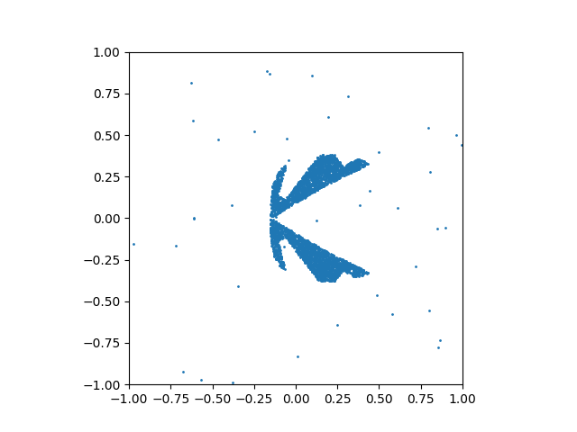
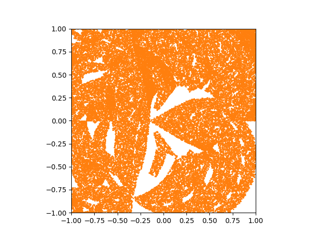
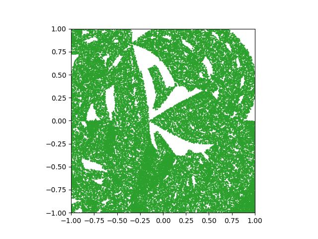
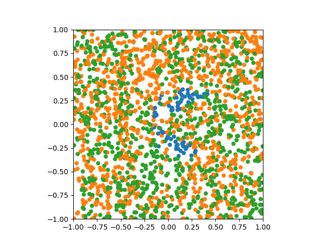
We’ll generate 2,000 random starting points for Laguerre’s method and color its location according to which root it converges to. Points converging to the real root are colored blue, points converging to the root with positive imaginary part are colored orange, and points converging to the root with negative imaginary part are colored green.

Here’s what we get:

This is hard to see, but we can tell that there aren’t many blue dots, about an equal number of orange and green dots, and the latter are thoroughly mixed together. This means the method is unlikely to converge to the real root, and about equally likely to converge to either of the complex roots.

Let’s look at just the starting points that converge to the real root, its basin of attraction. To get more resolution, we’ll generate 100,000 starting points and make the dots smaller.

The convergence region is pinched near the root; you can start fairly near the root along the real axis but converge to one of the complex roots. Notice also that there are scattered points far from the real root that converge to that point.

Next let’s look at the points that converge to the complex root in the upper half plane.

Note that the basin of attraction appears to take up over half the area. But the corresponding basin of attraction for the root in the lower half plane also appears to take up over half the area.

They can’t both take up over half the area. In fact. both take up about 48%. But the two regions are very intertwined. Due to the width of the dots used in plotting, each green dot covers a tiny bit of area that belongs to orange, and vice versa. That is, the fact that both appear to take over half the area shows how commingled they are.

Related posts

Breach Safe Harbor

In the context of medical data, Safe Harbor typically refers to the Safe Harbor provisions of the HIPAA Privacy Rule explained here. Breach Safe Harbor is a little different. It basically means you’re off the hook if you breach encrypted health data. (But not necessarily. More on that below.)

I’m not a lawyer, so this isn’t legal advice. Even the HHS, who coin the term “Breach Safe Harbor” in their guidance portal, weasels out of saying they’re giving legal guidance by saying “The contents of this database lack the force and effect of law, except as authorized by law …”

Quality of encryption

You can’t just say that data were encrypted before they were breached. Weak encryption won’t cut it. You have to use acceptable algorithms and procedures.

How can you know whether you’ve encrypted data well enough to be covered Breach Safe Harbor? HHS cites four NIST publications for further guidance. (Not that I’m giving legal advice. I’m merely citing the HHS, who also is not giving legal advice.)

Here are the four publications.

Maybe encryption isn’t enough

At one point Tennessee law said a breach of encrypted data was still a breach. According to Dempsey and Carlin [1]

In 2016, Tennessee repealed its encryption safe harbor, requiring notice of breach of even encrypted data, but then in 2017, after criticism, the state restored a safe harbor for “information that has been encrypted in accordance with the current version of the Federal Information Processing Standard (FIPS) 140-2 if the encryption key has not been acquired by an unauthorized person.”

This is interesting for a couple reasons. First, there is a precedent for requiring notification of encrypted data. Second, this underscores the point above that encryption in general is not sufficient to avoid having to give notice of a breach: standard-compliant encryption is sufficient.

Consulting help

If you would like technical or statistical advice on how to prevent or prepare for a data breach, or how to respond after a data breach after the fact, we can help.


[1] Jim Dempsey and John P. Carlin. Cybersecurity Law Fundamentals, Second Edition.

MD5 hash collision example

Marc Stevens gave an example of two alphanumeric strings that differ in only one byte that have the same MD5 hash value. It may seem like beating a dead horse to demonstrate weaknesses in MD5, but it’s instructive to study the flaws of broken methods. And despite the fact that MD5 has been broken for years, lawyers still use it.

The example claims that

TEXTCOLLBYfGiJUETHQ4hAcKSMd5zYpgqf1YRDhkmxHkhPWptrkoyz28wnI9V0aHeAuaKnak

and

TEXTCOLLBYfGiJUETHQ4hEcKSMd5zYpgqf1YRDhkmxHkhPWptrkoyz28wnI9V0aHeAuaKnak

have the same hash value.

This raises several questions.

Are these two strings really different, and if so, how do they differ? If you stare at the strings long enough you can see that they do indeed differ by one character. But how could you compare long strings like this in a more automated way?

How could you compute the MD5 hash values of the strings to verify that they are the same?

The following Python code addresses the questions above.

from hashlib import md5
from difflib import ndiff

def showdiff(a, b):
    for i,s in enumerate(ndiff(a, b)):
        if s[0]==' ': continue
        elif s[0]=='-':
            print(u'Delete "{}" from position {}'.format(s[-1],i))
        elif s[0]=='+':
            print(u'Add "{}" to position {}'.format(s[-1],i))    

a = "TEXTCOLLBYfGiJUETHQ4hAcKSMd5zYpgqf1YRDhkmxHkhPWptrkoyz28wnI9V0aHeAuaKnak"
b = "TEXTCOLLBYfGiJUETHQ4hEcKSMd5zYpgqf1YRDhkmxHkhPWptrkoyz28wnI9V0aHeAuaKnak"

showdiff(a, b)

ahash = md5(a.encode('utf-8')).hexdigest()
bhash = md5(b.encode('utf-8')).hexdigest()
assert(ahash == bhash)

The basis of the showdiff function was from an answer to a question on Stack Overflow.

The output of the call to showdiff is as follows.

Delete "A" from position 21
Add "E" to position 22

This means we can form string b from a by changing the ‘A’ in position 21 to an ‘E’. There was only one difference between the two strings in this example, but showdiff could be useful for understanding more complex differences.

The assert statement passes because both strings hash to faad49866e9498fc1719f5289e7a0269.

Related posts

Distance from a point to a line

Eric Lengyel’s new book Projective Geometric Algebra Illuminated arrived yesterday and I’m enjoying reading it. Imagine if someone started with ideas like dot products, cross products, and determinants that you might see in your first year of college, then thought deeply about those things for years. That’s kinda what the book is.

Early in the book is the example of finding the distance from a point q to a line of the form p + tv.

If you define u = q − p then a straightforward derivation shows that the distance d from q to the line is given by

d = \sqrt{{\bold u}^2 - \frac{({\bold u}\cdot {\bold v})^2}{{\bold v}^2}}

But as the author explains, it is better to calculate d by

d = \sqrt{\frac{({\bold u}\times {\bold v})^2}{{\bold v}^2}}

Why is that? The two expressions are algebraically equal, but the latter is better suited for numerical calculation.

The cardinal rule of numerical calculation is to avoid subtracting nearly equal floating point numbers. If two numbers agree to b bits, you may lose up to b bits of significance when computing their difference.

If u and v are vectors with large magnitude, but q is close to the line, then the first equation subtracts two large, nearly equal numbers under the square root.

The second equation involves subtraction too, but it’s less obvious. This is a common theme in numerical computing. Imagine this dialog.

[Student produces first equation.]

Mentor: Avoid subtracting nearly equal numbers.

[Student produces section equation.]

Student: OK, did it.

Mentor: That’s much better, though it could still have problems.

Where is there a subtraction in the second equation? We started with a subtraction in defining u. More subtly, the definition of cross product involves subtractions. But these subtractions involve smaller numbers than the first formula, because the first formula subtracts squared values. Eric Lengyel points this out in his book.

None of this may matter in practice, until it does matter, which is a common pattern in numerical computing. You implement something like the first formula, something that can be derived directly. You implicitly have in mind vectors whose magnitude is comparable to d and this guides your choice of unit tests, which all pass.

Some time goes by and a colleague tells you your code is failing. Impossible! You checked your derivation by hand and in Mathematica. Your unit tests all pass. Must be your colleague’s fault. But it’s not. Your code would be correct in infinite precision, but in an actual computer it fails on inputs that violate your implicit assumptions.

This can be frustrating, but it can also be fun. Implementing equations from a freshman textbook accurately, efficiently, and robustly is not a freshman-level exercise.

Related posts

Experiences with Thread Programming in Microsoft Windows

Lately I’ve been helping a colleague to add worker threads to his GUI-based Windows application.

Thread programming can be tricky. Here are a few things I’ve learned along the way.

Performance. This app does compute-intensive work. It is helpful to offload this very compute-heavy work to a worker thread. Doing this frees the main thread to service GUI requests better.

Thread libraries. Windows has multiple thread libraries, for example Microsoft Foundation Class library threads and C++ standard library threads. It is hazardous to use different thread libraries in the same app. In the extreme case, different thread libraries, such as GOMP  vs. LOMP, used in resp. the GCC and LLVM compiler families, have different threading runtimes which keep track of threads in different ways. Mixing them in the same code can cause hazardous silent errors.

Memory fences are a thing. Different threads can run on different processor cores and hold variables in different respective L1 caches that are not flushed (this to maintain high performance). An update to a variable by one thread is not guaranteed to be visible to other threads without special measures. For example, one could safely transfer information using ::PostMessage coupled with a handler function on the receiver thread. Or one could send a signal using an MFC CEvent on one thread and read its Lock on the other. Also, a thread launch implicitly does a memory fence, so that, at least then, the new thread is guaranteed to correctly see the state of all memory locations.

GUI access should be done from the master thread only, not a worker thread. Doing so can result in deadlock. A worker thread can instead ::PostMessage to ask the master thread to do a GUI action.

Thread launch. By default AfxBeginThread returns a thread handle which MFC takes care of deleting when no longer needed. If you want to manage the life cycle of the handle yourself, you can do something like:

myWorkerThreadHandle = AfxBeginThread(myFunc, myParams,
  THREAD_PRIORITY_NORMAL, 0, CREATE_SUSPENDED);
myWorkerThreadHandle->m_bAutoDelete = false;
myWorkerThreadHandle->ResumeThread();

Joint use of a shared library like the DAO database library has hazards. One should beware of using the library to allocate something in one thread and deallocating in another, as this will likely allocate in a thread-local heap or stack instead of a shared thread-safe heap, this resulting in a crash.

Initialization. One should call CoInitializeEx(NULL, COINIT_APARTMENTTHREADED) and AfxDaoInit() (if using DAO) at thread initialization on both master and worker threads, and correspondingly CoUninitialize() and AfxDaoTerm() at completion of the thread.

Monitoring of thread state can be done with
WaitForSingleObject(myWorkerThreadHandle->m_hThread, 0) to determine if the thread has completed or WaitForSingleObject(myWorkerThreadHandle->m_hThread, INFINITE) for a blocking wait until completion.

Race conditions are always a risk but can be avoided by careful reasoning about execution. Someone once said up to 90% of code errors can be found by desk checking [1]. Race conditions are notoriously hard to debug, partly because they can occur nondeterministically. There are tools for trying to find race condition errors, though I’ve never tried them.

So far I find no rigorous specification of the MFC threading model online that touches on all these concerns. Hopefully this post is useful to someone else working through these issues.

References

[1] Dasso, Aristides., Funes, Ana. Verification, Validation and Testing in Software Engineering. United Kingdom: Idea Group Pub., 2007, p. 163.

Accelerating Archimedes

One way to approximate π is to find the areas of polygons inscribed inside a circle and polygons circumscribed outside the circle. The approximation improves as the number of sides in the polygons increases. This idea goes back at least as far as Archimedes (287–212 BC). Maybe you’ve tried this. It’s a lot of work.

In 1667 James Gregory came up with a more efficient way to carry out Archimedes’ approach. Tom Edgar and David Richeson cite Gregory’s theorem in [1] as follows.

Let Ik and Ck denote the areas of regular k-gons inscribed in and circumscribed around a given circle. Then I2n is the geometric mean of In and Ck, and C2n is the harmonic mean of I2n and Cn; that is,

\begin{align*} I_{2n} &= \sqrt{I_nC_n} \\ C_{2n} &= \frac{2C_n I_{2n}}{C_n + I_{2n}} \end{align*}

We can start with n = 4. Obviously the square circumscribed around the unit circle has vertices at (±1, ±1) and area 4. A little thought finds that the inscribed square has vertices at (±√2/2, ±√2/2) and area 2.

The following Python script finds π to six decimal places.

n = 4
I, C = 2, 4 # inscribed area, circumscribed area
delta = 2

while delta > 1e-6:
    I = (I*C)**0.5
    C = 2*C*I / (C + I)
    delta = C - I
    n *= 2
    print(n, I, C, delta)

The script stops when n = 8192, meaning that the difference between the areas of an inscribed and circumscribed 8192-gon is less than 10−6. The final output of the script is.

8192 3.1415923 3.1415928 4.620295e-07

If we average the upper and lower bound we get one more decimal place of accuracy.

Gregory’s algorithm isn’t fast, though it’s much faster than carrying out Archimedes’ approach by computing each area from scratch.

Gregory gives an interesting recursion. It has an asymmetry that surprised me: you update I, then C. You don’t update them simultaneously as you do when you’re computing the arithmetic-geometric mean.

Related posts

[1] Tom Edgar and David Richeson. A Visual Proof of Gregory’s Theorem. Mathematics Magazine, December 2019, Vol. 92, No. 5 (December 2019), pp. 384–386

How much will a cable sag? A simple approximation

Suppose you have a cable of length 2s suspended from two poles of equal height a distance 2x apart. Assuming the cable hangs in the shape of a catenary, how much does it sag in the middle?

If the cable were pulled perfectly taut, we would have s = x and there would be no sag. But in general, s > x and the cable is somewhat lower in the middle than on the two ends. The sag is the difference between the height at the end points and the height in the middle.

The equation of a catenary is

y = a cosh(t/a)

and the length of the catenary between t = −x and t = x is

2s = 2a sinh(x/a).

You could solve this equation for a and the sag will be

g = a cosh(x/a) − a.

Solving for a given s is not an insurmountable problem, but there is a simple approximation for g that has an error of less than 1%. This approximation, given in [1], is

g² = (s − x)(sx/2).

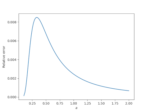
To visualize the error, I set x = 1 and let a vary to produce the plot below.

The relative error is always less than 1/117. It peaks somewhere around x = 1/3 and decreases from there, the error getting smaller as a increases (i.e. the cable is pulled tighter).

Related posts

[1] J. S. Frame. An approximation for the dip of a catenary. Pi Mu Epsilon Journal, Vol. 1, No. 2 (April 1950), pp. 44–46

Unique letter patterns in words

The word Mississippi has a unique pattern of letters. If you were solving a cryptogram puzzle and saw ZVFFVFFVCCV you might guess that the word is Mississippi.

Is the pattern of letters in Mississippi literally unique or just uncommon? What is the shortest word with a unique letter pattern? The longest word?

We can answer these questions by looking at normalized cryptograms, a sort of word signature. These are formed by replacing the first letter in a word with ‘A’, the next unique letter with ‘B’, etc. The normalized cryptogram of Mississippi is ABCCBCCBDDB.

The set of English words is fuzzy, but for my purposes I will take “words” to mean the entries in the dictionary file american-english on my Linux box, removing words that contain apostrophes or triple letters. I computed the cryptogram of each word, then looked for those that only appear once.

Relative to the list of words I used, yes, Mississippi is unique.

The shortest word with a unique cryptogram is eerie. [1]

The longest word with a unique cryptogram is ambidextrously. Every letter in this 14-letter word appears only once.

[1] Update: eerie is a five-letter example, but there are more. Jack Kennedy pointed out amass, llama, and mamma in the comments. I noticed eerie because its cryptogram comes first in alphabetical order.

How to Organize Technical Research?


64 million scientific papers have been published since 1996 [1].

Assuming you can actually find the information you want in the first place—how can you organize your findings to be able to recall and use them later?

It’s not a trifling question. Discoveries often come from uniting different obscure pieces of information in a new way, possibly from very disparate sources.

Many software tools are used today for notetaking and organizing information, including simple text files and folders, Evernote, GitHub, wikis, Miro, mymind, Synthical and Notion—to name a diverse few.

AI tools can help, though they can’t always recall correctly and get it right, and their ability to find connections between ideas is elementary. But they are getting better [2,3].

One perspective was presented by Jared O’Neal of Argonne National Laboratory, from the standpoint of laboratory notebooks used by teams of experimental scientists [4]. His experience was that as problems become more complex and larger, researchers must invent new tools and processes to cope with the complexity—thus “reinventing the lab notebook.”

While acknowledging the value of paper notebooks, he found electronic methods essential because of distributed teammates. In his view many streams of notes are probably necessary, using tools such as GitLab and Jupyter notebooks. Crucial is the actual discipline and methodology of notetaking, for example a hierarchical organization of notes (separating high-level overview and low-level details) that are carefully written to be understandable to others.

A totally different case is the research methodology of 19th century scientist Michael Faraday. He is not to be taken lightly, being called by some “the best experimentalist in the history of science” (and so, perhaps, even compared to today) [5].

A fascinating paper [6] documents Faraday’s development of “a highly structured set of retrieval strategies as dynamic aids during his scientific research.” He recorded a staggering 30,000 experiments over his lifetime. He used 12 different kinds of record-keeping media, including lab notebooks proper, idea books, loose slips, retrieval sheets and work sheets. Often he would combine ideas from different slips of paper to organize his discoveries. Notably, his process to some degree varied over his lifetime.

Certain motifs emerge from these examples: the value of well-organized notes as memory aids; the need to thoughtfully innovate one’s notetaking methods to find what works best; the freedom to use multiple media, not restricted to a single notetaking tool or format.

Do you have a favorite method for organizing your research? If so, please share in the comments below.

References

[1] How Many Journal Articles Have Been Published? https://publishingstate.com/how-many-journal-articles-have-been-published/2023/

[2] “Multimodal prompting with a 44-minute movie | Gemini 1.5 Pro Demo,” https://www.youtube.com/watch?v=wa0MT8OwHuk

[3] Geoffrey Hinton, “CBMM10 Panel: Research on Intelligence in the Age of AI,” https://www.youtube.com/watch?v=Gg-w_n9NJIE&t=4706s

[4] Jared O’Neal, “Lab Notebooks For Computational Mathematics, Sciences, Engineering: One Ex-experimentalist’s Perspective,” Dec. 14, 2022, https://www.exascaleproject.org/event/labnotebooks/

[5] “Michael Faraday,” https://dlab.epfl.ch/wikispeedia/wpcd/wp/m/Michael_Faraday.htm

[6] Tweney, R.D. and Ayala, C.D., 2015. Memory and the construction of scientific meaning: Michael Faraday’s use of notebooks and records. Memory Studies8(4), pp.422-439. https://www.researchgate.net/profile/Ryan-Tweney/publication/279216243_Memory_and_the_construction_of_scientific_meaning_Michael_Faraday’s_use_of_notebooks_and_records/links/5783aac708ae3f355b4a1ca5/Memory-and-the-construction-of-scientific-meaning-Michael-Faradays-use-of-notebooks-and-records.pdf