Example of the bike shed principle

Celebration, Florida town seal

One of the case studies in Michael Beirut’s book How to is the graphic design for the planned community Celebration, Florida. The logo for the town’s golf course is an illustration of the bike shed principle.

C. Northcote Parkinson observed that it is easier for a committee to approve a nuclear power plant than a bicycle shed. Nuclear power plants are complex, and no one on a committee presumes to understand every detail. Committee members must rely on the judgment of others. But everyone understands bicycle sheds. Also, questions such as what color to paint the bike shed don’t have objective answers. And so bike sheds provoke long discussions.

People argue about bike sheds because they understand bike sheds. Beirut said something similar about the Celebration Golf Club logo which features a silhouette of a golfer.

Designing the graphics for Celebration’s public golf club was much harder than designing the town seal. It took me some time to realize why: none of our clients were Schwinn-riding, polytailed girls [as in the town seal], but most of them were enthusiastic golfers. The silhouette on the golf club design was refined endlessly as various executives demonstrated their swings in client meetings.

Image credit: By Source, Fair use, https://en.wikipedia.org/w/index.php?curid=37643922

Plastic powers

Last week I wrote a blog post showing that powers of the golden ratio are nearly integers. Specifically, the distance from φn to the nearest integer decreases exponentially as n increases. Several people pointed out that the golden constant is a Pisot number, the general class of numbers whose powers are exponentially close to integers.

The so-called plastic constant P is another Pisot number, in fact the smallest Pisot number. P is the real root of x3x − 1 = 0.

P = \frac{ (9 - \sqrt{69})^{1/3} + (9 + \sqrt{69})^{1/3} }{ 2^{1/3} \,\,\, 3^{2/3} } = 1.3247\ldots

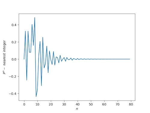
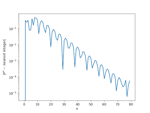
Because P is a Pisot number, we know that its powers will be close to integers, just like powers of the golden ratio, but the way they approach integers is more interesting. The convergence is slower and less regular.

We will the first few powers of P, first looking at the distance to the nearest integer on a linear scale, then looking at the absolute value of the distance on a logarithmic scale.

distance from powers of plastic constant to nearest integer

distance from powers of plastic constant to nearest integer, log scale

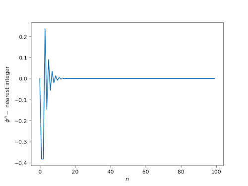
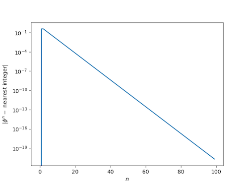
As a reminder, here’s what the corresponding plots looked like for the golden ratio.

distance from powers of golden ratio to nearest integer

distance from powers of golden ratio to nearest integer, log scale

Visualizing kinds of rings

When I first saw ring theory, my impression was that there were dozens of kinds of rings with dozens of special relations between them—more than I could keep up with. In reality, there just a few basic kinds of rings, and the relations between them are simple.

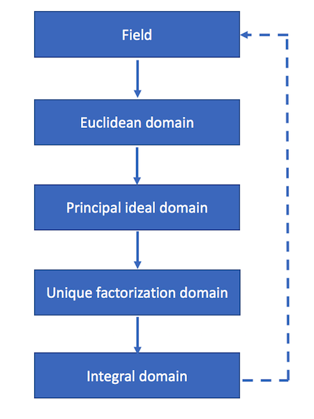
Here’s a diagram that shows the basic kinds of rings and the relations between them. (I’m only looking at commutative rings, and I assume ever ring has a multiplicative identity.)

Types of commutative rings

The solid lines are unconditional implications. The dashed line is a conditional implication.

  • Every field is a Euclidean domain.
  • Every Euclidean domain is a principal ideal domain (PID).
  • Every principal ideal domain is a unique factorization domain (UFD).
  • Every unique factorization domain is an integral domain.
  • A finite integral domain is a field.

Incidentally, the diagram has a sort of embedded pun: the implications form a circle, i.e. a ring.

More mathematical diagrams:

Freudian hypothesis testing

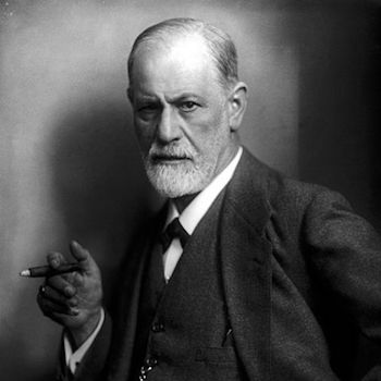
Sigmund Freud

In his paper Mindless statistics, Gerd Gigerenzer uses a Freudian analogy to describe the mental conflict researchers experience over statistical hypothesis testing. He says that the “statistical ritual” of NHST (null hypothesis significance testing) “is a form of conflict resolution, like compulsive hand washing.”

In Gigerenzer’s analogy, the id represents Bayesian analysis. Deep down, a researcher wants to know the probabilities of hypotheses being true. This is something that Bayesian statistics makes possible, but more conventional frequentist statistics does not.

The ego represents R. A. Fisher’s significance testing: specify a null hypothesis only, not an alternative, and report a p-value. Significance is calculated after collecting the data. This makes it easy to publish papers. The researcher never clearly states his hypothesis, and yet takes credit for having established it after rejecting the null. This leads to feelings of guilt and shame.

The superego represents the Neyman-Pearson version of hypothesis testing: pre-specified alternative hypotheses, power and sample size calculations, etc. Neyman and Pearson insist that hypothesis testing is about what to do, not what to believe. [1]

I assume Gigerenzer doesn’t take this analogy too seriously. In context, it’s a humorous interlude in his polemic against rote statistical ritual.

But there really is a conflict in hypothesis testing. Researchers naturally think in Bayesian terms, and interpret frequentist results as if they were Bayesian. They really do want probabilities associated with hypotheses, and will imagine they have them even though frequentist theory explicitly forbids this. The rest of the analogy, comparing the ego and superego to Fisher and Neyman-Pearson respectively, seems weaker to me. But I suppose you could imagine Neyman and Pearson playing the role of your conscience, making you feel guilty about the pragmatic but unprincipled use of p-values.

* * *

[1] “No test based upon a theory of probability can by itself provide any valuable evidence of the truth or falsehood of a hypothesis. But we may look at the purpose of tests from another viewpoint. Without hoping to know whether each separate hypothesis is true or false, we may search for rules to govern behaviour in regard to them, in following which we insure that, in the long run of experience, we shall not often be wrong.”

Neyman J, Pearson E. On the problem of the most efficient tests of statistical hypotheses. Philos Trans Roy Soc A, 1933;231:289, 337.

Golden powers are nearly integers

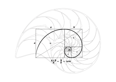
Nautilus, golden ratio

This morning I was reading Terry Tao’s overview of the work of Yves Meyer and ran across this line:

The powers φ, φ2, φ3, … of the golden ratio lie unexpectedly close to integers: for instance, φ11 = 199.005… is unusually close to 199.

I’d never heard that before, so I wrote a little code to see just how close golden powers are to integers.

Here’s a plot of the difference between φn and the nearest integer:

distance from powers of golden ratio to nearest integer

(Note that if you want to try this yourself, you need extended precision. Otherwise you’ll get strange numerical artifacts once φn is too large to represent exactly.)

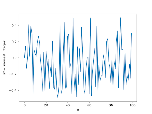
By contrast, if we make the analogous plot replacing φ with π we see that the distance to the nearest integer looks like a uniform random variable:

distance from powers of pi to nearest integer

The distance from powers of φ to the nearest integer decreases so fast that cannot see it in the graph for moderate sized n, which suggests we plot the difference on the log scale. (In fact we plot the log of the absolute value of the difference since the difference could be negative and the log undefined.) Here’s what we get:

absolute distance from powers of golden ratio to nearest integer on log scale

After an initial rise, the curve is apparently a straight line on a log scale, i.e. the absolute distance to the nearest integer decreases almost exactly exponentially.

Related math posts

Antidepressants for van Gogh

Van Gogh stamp

In a recent interview, Tyler Cowen discusses complacency, (neruo-)diversity, etc.

Let me give you a time machine and send you back to Vincent van Gogh, and you have some antidepressants to make him better. What actually would you do, should you do, could you do? We really don’t know. Maybe he would have had a much longer life and produced more wonderful paintings. But I worry about the answer to that question.

And I think in general, for all the talk about diversity, we’re grossly undervaluing actual human diversity and actual diversity of opinion. Ways in which people—they can be racial or ethnic but they don’t have to be at all—ways in which people are actually diverse, and obliterating them somewhat. This is my Toquevillian worry and I think we’ve engaged in the massive social experiment of a lot more anti-depressants and I think we don’t know what the consequences are. I’m not saying people shouldn’t do it. I’m not trying to offer any kind of advice or lecture.

I don’t share Cowen’s concern regarding antidepressants. I haven’t thought about it before. But I am concerned with how much we drug restless boys into submission. (Girls too, of course, but it’s usually boys.)

Duals and double duals of Banach spaces

The canonical examples of natural and unnatural transformations come from linear algebra, namely the relation between a vector space and its first and second duals. We will look briefly at the finite dimensional case, then concentrate on the infinite dimensional case.

Two finite-dimensional vector spaces over the same field are isomorphic if and only if they have the same dimension.

For a finite dimensional space V, its dual space V* is defined to be the vector space of linear functionals on V, that is, the set of linear functions from V to the underlying field. The space V* has the same dimension as V, and so the two spaces are isomorphic. You can do the same thing again, taking the dual of the dual, to get V**. This also has the same dimension, and so V is isomorphic to V** as well as V*. However, V is naturally isomorphic to V** but not to V*. That is, the transformation from V to V* is not natural.

Some things in linear algebra are easier to see in infinite dimensions, i.e. in Banach spaces. Distinctions that seem pedantic in finite dimensions clearly matter in infinite dimensions.

The category of Banach spaces considers linear spaces and continuous linear transformations between them. In a finite dimensional Euclidean space, all linear transformations are continuous, but in infinite dimensions a linear transformation is not necessarily continuous.

The dual of a Banach space V is the space of continuous linear functions on V. Now we can see examples of where not only is V* not naturally isomorphic to V, it’s not isomorphic at all.

For any real p > 1, let q be the number such that 1/p  + 1/q = 1. The Banach space Lp is defined to be the set of (equivalence classes of) Lebesgue integrable functions f such that the integral of |f|p is finite. The dual space of Lp is Lq. If p does not equal 2, then these two spaces are different. (If p does equal 2, then so does qL2 is a Hilbert space and its dual is indeed the same space.)

In the finite dimensional case, a vector space V is isomorphic to its second dual V**. In general, V can be embedded into V**, but V** might be a larger space. The embedding of V in V** is natural, both in the intuitive sense and in the formal sense of natural transformations, discussed in the previous post. We can turn an element of V into a linear functional on linear functions on V as follows.

Let v be an element of V and let f be an element of V*. The action of v on f is simply fv. That is, v acts on linear functions by letting them act on it!

This shows that some elements of V** come from evaluation at elements of V, but there could be more. Returning to the example of Lebesgue spaces above, the dual of L1 is L, the space of essentially bounded functions. But the dual of L is larger than L1. That is, one way to construct a continuous linear functional on bounded functions is to multiply them by an absolutely integrable function and integrate. But there are other ways to construct linear functionals on L.

A Banach space V is reflexive if the natural embedding of V in V** is an isomorphism. For p > 1, the spaces Lp are reflexive.

However, R. C. James proved the surprising result that there are Banach spaces that are isomorphic to their second duals, but not naturally. That is, there are spaces V where V is isomorphic to V**, but not via the natural embedding; the natural embedding of V into V** is not an isomorphism.

Related: Applied functional analysis

Natural transformations

The ladder of abstractions in category theory starts with categories, then functors, then natural transformations. Unfortunately, natural transformations don’t seem very natural when you first see the definition. This is ironic since the original motivation for developing category theory was to formalize the intuitive notion of a transformation being “natural.” Historically, functors were defined in order to define natural transformations, and categories were defined in order to define functors, just the opposite of the order in which they are introduced now.

A category is a collection of objects and arrows between objects. Usually these “arrows” are functions, but in general they don’t have to be.

A functor maps a category to another category. Since a category consists of objects and arrows, a functor maps objects to objects and arrows to arrows.

A natural transformation maps functors to functors. Sounds reasonable, but what does that mean?

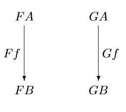
You can think of a functor as a way to create a picture of one category inside another. Suppose you have some category and pick out two objects in that category, A and B, and suppose there is an arrow f between A and B. Then a functor F would take A and B and give you objects FA and FB in another category, and an arrow Ff between FA and FB. You could do the same with another functor G. So the objects A and B and the arrow between them in the first category have counterparts under the functors F and G in the new category as in the two diagrams below.

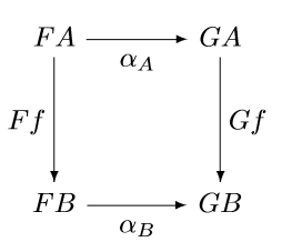
A natural transformation α between F and G is something that connects these two diagrams into one diagram that commutes.

The natural transformation α is a collection of arrows in the new category, one for every object in the original category. So we have an arrow αA for the object A and another arrow αB for the object B. These arrows are called the components of α at A and B respectively.

Note that the components of α depend on the objects A and B but not on the arrow f. If f represents any other arrow from A to B in the original category, the same arrows αA and αB fill in the diagram.

Natural transformations are meant to capture the idea that a transformation is “natural” in the sense of not depending on any arbitrary choices. If a transformation does depend on arbitrary choices, the arrows αA and αB would not be reusable but would have to change when f changes.

The next post will discuss the canonical examples of natural and unnatural transformations.

Related posts