Dual axioms in modal logic

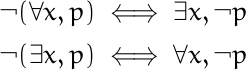
Axioms in modal logic often say that one sequence of boxes and diamonds in front of a proposition p implies another sequence of boxes and diamonds in front of p. For example, Axiom 4 says

p → □□ p

and Axiom 5 says

p → □◇p.

Every axiom has a dual form. The dual form of Axiom 4 is

◇◇p → ◇p

and the dual of Axiom 5 is

◇□ p → □ p.

Computing duals

There’s a simple way to compute the dual of such axioms:

Rotate all the squares 45° and rotate the arrow 180°.

This turns boxes into diamonds, diamonds into boxes, and flips the direction of implication.

Shell and Perl

We could do this using the tr utility at the command line

    $ echo '□□◇□◇p → □◇p' | tr '□◇→' '◇□←'
    ◇◇□◇□p ← ◇□p

We could also do the same thing in Perl, using its tr operator

    $prop = "□□◇□◇p → □◇p";
    ($dual = $prop) =~ tr/□◇→/◇□←/;
    print "$prop\n$dual\n";

This prints

    □□◇□◇p → □◇p
    ◇◇□◇□p ← ◇□p

It’s important to note that tr in both its incarnations does simultaneous replacement. It did what we expected, so it might be hard to notice.

tr takes two strings of the same length as arguments. Call the first one from and the second to. The easiest way to implement tr would have been to replace the first character of from with the first character of to, then replace the second character of from with the second character of to, etc.

This would have turned all our boxes into diamonds, then turned all diamonds into boxes, and so we’d be left with nothing but boxes! Our sequence □□◇□◇ would have turned into □□□□□.

Proof

Why is the rule above valid?

Let ○ stand for either a box or a diamond and suppose we start with

12 … ○m p → ○m+1m+2 … ○n p

where p is an arbitrary proposition.

Now let ○’ stand for the dual of ○. So if ○ is a box, ○’ is a diamond, and vice versa. Then

○ p = ¬○’ ¬p

by definition. (If you take □ as primary, then the equation above is the definition of ◇. If you take ◇ as primary, it’s the definition of □.) Apply this rule everywhere.

¬○’1 ¬¬○’2 ¬… ¬○’m ¬p → ¬○’m+1 ¬¬○’m+2 … ¬○’n ¬p

Now cancel out all the pairs of consecutive negations.

¬○’1 ○’2 … ○’m ¬p → ¬○’m+1 ○’m+2 … ○’n ¬p

Now take the contrapositive: (¬P → ¬Q) → (QP).

○’m+1 ○’m+2 … ○’n ¬p → ○’1 ○’2 … ○’m ¬p

Since p was an arbitrary proposition, we can replace p with ¬p.

○’m+1 ○’m+2 … ○’n p → ○’1 ○’2 … ○’m p

What we have above is the proposition we started with, with all the boxes replaced with diamonds, all the diamonds replaced with boxes, and the direction of the implication reversed.

More modalities

Notice that the theorem and proof still holds if there are multiple modalities. Suppose we have a set of modalities Ki. You could interpret

Ki p

as saying the ith agent knows proposition p is true. Then the dual is defined by

K’i p = ¬ Ki ¬ p,

which could be interpreted as saying the ith agent does not know p to be false.

You could form the dual of a proposition involving K and K‘ expressions by adding primes to terms that don’t have them, and removing primes from terms that do, and turning the implication around. The proof would be the same as above, only we don’t restrict ○ to being □ or ◇.
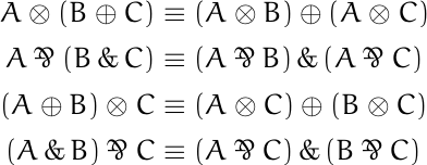
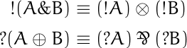
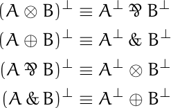
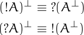
Related posts

Word problems, logic, and regular expressions

Word problems

Suppose you have a sequence of symbols and a set of rewriting rules for replacing some patterns of symbols with others. Now you’re given two such sequences. Can you tell whether there’s a way to turn one of them into the other?

This is known as the word problem, and in general it’s undecidable. In general the problem cannot be solved by a program, but some instances can. We’ll look at a word problem that can be solved with a few regular expressions.

Modal logic

Basic modal logic has two symbols, □ (“box”) and ◇ (“diamond”), and concatenations of these symbols. In general, there are infinitely many non-equivalent sequences of boxes and diamonds, depending on the axioms of your modal logic.

In the axiom system S4, every non-empty sequence of boxes and diamonds is equivalent to one of six possibilities:

  • □◇
  • ◇□
  • □◇□
  • ◇□◇

An arbitrary sequence of boxes and diamonds can be reduced to one of the forms above by applying the following rules:

  • □ □ → □
  • ◇ ◇ → ◇
  • □◇□◇ → □◇
  • ◇□◇□ → ◇□

Regular expressions

We can apply the reduction rules above using regular expressions with the following Perl code.

    use utf8;

    $_ = "□□◇□◇◇◇◇□□";

    s/□+/□/g;
    s/◇+/◇/g; 
    s/(□◇)+/□◇/g; 
    s/(◇□)+/◇□/g;

    print;

The directive use utf8; tells Perl to be prepared for non-ASCII characters, namely boxes and diamonds. In Perl, $_ is the implicit variable; all the following substitution commands will modify this variable, and the print statement will output the final value of this variable.

The first substitution replaces one or more consecutive boxes with one box and the second does the analogous substitution for consecutive diamonds. The third and fourth substitution commands replace repetitions of □◇ or ◇□ with a single instance.

The script above outputs

□◇□

meaning that

□□◇□◇◇◇◇□□p ⟷ □◇□p

is a theorem in S4.

Word problems can’t always be solved using regular expressions, or any other programming technique, but this one could.

Related posts

Modal axioms and rules for interplanetary travel

The previous post pointed out the analogy between models for modal logic (i.e. Kripke semantics) and science fiction. Rules for relationships between points in a Kripke model are analogous to rules for interplanetary travel in a fictional universe. This post will expand on this last point.

The following cube shows the relationships between eight different axiom systems for modal logic. Unfortunately, as I’ve written about before, the names of these systems are more historical than mnemonic.

Modal logic axiom cube

An arrow from A to B means the set of propositions provable in A contain the propositions provable in B.

For example, all the systems represent by the cube are “normal,” meaning that they all require Axiom K. So any proposition provable in K is provable in the other systems as well.

The axes of the cube correspond to rules for how “worlds” are connected in Kripke models. Imagine that K in the diagram is the origin. The x axis (from K to KB) corresponds to symmetry, the y axis (from K to K4) corresponds to transitivity, and the z axis (from K to T) corresponds to reflexivity.

S4 example

S4 in the diagram has coordinates (0, 1, 1), meaning that Kripke models for S4 must be transitive and reflexive. In SF terms, this says you can travel from any planet back to itself, and if it is possible to travel from planet x to planet y, and possible to travel from planet y to planet z, then it must be possible to travel from x to y.

Why weaker systems than S5?

Models of S5 are symmetric: if you can travel from x to y, you can travel from y to x. S4 does not have this requirement.

The axioms for S5 seem so sensible that you may wonder what the point is in having weaker systems. It all depends on how you interpret the modal qualifier □. In some applications of modal logic, □ has properties that correspond to models with unusual restrictions on accessibility.

We’re not trying to use logic to describe networks, though we could, but rather creating networks to model systems of logic. The resulting networks may have strange geometry if they weren’t motivated by geometry to begin with.

Axiom K

Axiom K (named for Saul Kripke) requires that

□(p → q) →  (□p → □q)

This says that if the proposition p → q is true in all accessible worlds, and if p is true in all accessible worlds, then q must be true in all accessible worlds.

Axiom T

Axiom T requires that

p →p.

If something is true in all worlds accessible from a world w, and w is accessible from itself, then it must be true on w.

Axiom 4

Axiom 4 requires

p → □□p.

Standing on a world w, the proposition □p says that p is true on all worlds accessible from w. So if x is a world accessible from w, p is true there. And if y is a world accessible from x, then by transitivity that world must be accessible from x, so p is true there. So □p is true on x. And since □p is true on any world accessible from w, then we can say □□p.

Axiom B

Axiom B requires

p → □◇p.

One way to state this is that if a proposition is true, then it is necessarily possibly true.

Imagine you’re on a world w there p is true. Symmetry says that if a world x accessible from w, then w is accessible from x. Now □◇p holds because in any world x accessible from w, we have ◇p because w is accessible from x.

Axiom 5

Axiom 5 requires

p →□◇p.

In words, whatever is possible is necessarily possible. A Kripke model for axiom 5 must be Euclidean: If from world w you can access worlds x and y, then from x you can access y. A relation that is symmetric and transitive is Euclidean. If x is accessible from w, then symmetry says w is accessible from x, and transitivity says you can go on from w to y.

Systems versus Axioms

One of the confusing things about modal logic is the complicated relation between the names of axioms and systems of axioms. Sometimes it’s simple. For example, K4 means the system with axioms K and 4.

The vertices of the cube above are systems, not axioms. And system B, confusingly, requires more than axiom B, and is in fact stronger than system KB because it adds axiom T. Chellas [1] calls this system KTB, a more verbose but more transparent name.

Provenance of the cube

The cube at the top of this post is a simplification of similar diagrams that appear in The Standford Encyclopedia of Philosophy and Wikipedia. Both may trace their origin to figure 4.1 in [1]. I don’t know that either diagram came from there, or whether they were developed independently, but [1] predates both. However, the graph in Chellas is less clear. The edge directions are implicit, as is the connection to properties of the models.

Related posts

[1] Brian F. Chellas. Modal Logic: An Introduction. 1980,

Modal Logic and Science Fiction

Astronauts exploring an asteroid

Modal logic extends classical logic by adding one or more modes. If there’s only one mode, it’s usually denoted □. Curiously,  □ can have a wide variety of interpretations, and different interpretations motivate different axioms for how □ behaves. Modal logic is not one system but an infinite number of systems, depending on your choice of axioms, though a small number of axiom systems come up in application far more than others.

For a proposition p, □p is often interpreted as “necessarily p” but it could also be read, for example, as “it is provable that p“. Thanks to Gödel, we know some theorems are true but not provable, so p might be true while □p is false.

Kripke semantics interprets □p to be true at a “worldw if p is true in all worlds accessible from w. The rules of a logic system transfer to and from the set of models for that system, where a model is a directed graph of worlds, and an oracle (a “valuation function”) that tells you what’s true on each world. Axioms for a logic system correspond to requirements regarding the connectivity of all graph models for the system.

All this talk of what worlds are accessible from other worlds sounds a lot like science fiction. For example, if the planet Vulcan is accessible from Earth, and p is the statement “The blood of sentient beings is red,” then p is true on Earth, but not necessarily true on Earth since it’s not true on Vulcan, a world accessible from Earth.

Modal logic defines ◇ by

p = ¬ □ ¬ p.

For a proposition p, ◇p can be read as “possibly p.” A proposition ◇p is true on a world w if there is some world accessible from w where p is true.

So in the Star Trek universe, if p is the statement “Blood is green” then p is false on Earth, and so is □p, but ◇p is true because there is a world accessible from earth, namely Vulcan, where p is true.

You could have all kinds of fun making up rules about which worlds are accessible from each other. If someone from planet x can reach planet y, and someone from planet y can reach planet z, can someone from x reach z? Sounds reasonable, and if all worlds have this property then your Kripke frame is said to be transitive. But you could create a fictional universe in which, for whatever reason, this doesn’t hold.

Is a world accessible from itself? Depends on how you define accessibility. You might decide that a non-space faring world is not accessible from itself. But if every world is accessible from itself, your Kripke model is reflexive. If a Kripke frame is reflexive and transitive, the corresponding logic satisfies the S4 axioms. (More on this in the next post.)

Johan van Benthem gives an example in his book Modal Logic for Open Minds that’s scientific but not fictional. If you define a “world” to be a point in Minkowski space-time, then the worlds accessible from a given world are in that world’s future light cone. Propositions in this logic satisfy

◇□ p →□◇ p

and in fact the logic satisfies a system of axioms known as S4.2.

More modal logic posts

Reading plots of a complex function

This post is about understanding the following plot. If you’d like to read more along these lines, see [1].

Hankel function phase plot

The plot was made with the following Mathematica command.

    ComplexPlot[HankelH1[3, z], {z, -8 - 4 I, 4 + 4 I}, 
        ColorFunction -> "CyclicArg", AspectRatio -> 1/2]

The plot uses color to represent the phase of the function values. If the output of the function is written in polar form as (r, θ), we’re seeing θ.

Here’s a plot of the identity function f(z) = z to show how the color rotation works.

The color rotate from red to orange to green etc. (ROYGBIV) clockwise around a pole and counterclockwise around a zero.

You can see from the plot at the top that our function has a pole at 0. In fact, it’s a pole of order three because you go through the ROYGBIV cycle three times clockwise as you circle the origin.

You can also see four zeros, located near −6.4 − 0.4i, −2, 2 − i, −0.4 − 2i, and −1.3 − 1.7i. In each case we cycle through ROYGBIV one time counterclockwise, so these are simple zeros. If we had a double zero, we’d cycle through the colors twice. If we had a triple zero, we’d cycle through the colors three times, just as we did at the pole, except we’d go through the colors counterclockwise.

The colors in our plot vary continuously, except on the left side. There’s a discontinuity in our colors above and below the real axis. That’s because the function we’re plotting has a branch cut from −∞ to 0. The discontinuity isn’t noticeable near the origin, but it becomes more noticeable as you move away from the origin to the left.

Here’s a 3D plot to let us see the branch cut more clearly.

Here color represents phase as before, but now height represents absolute value, the r in our polar representation. The flat plateau on top is an artifact. The function becomes infinite at 0, so it had to be cut off.

You can see a seam in the graph. There’s a jump discontinuity along the negative real axis, with the function taking different values as you approach the real axis from the second quadrant or from the third quadrant.

This came up in a previous post, Architecture and math, but I didn’t say anything about it. Here’s a plot from that post.

Why is there a little radial line on top where the graph was chopped off? And why is there a white streak below it? That’s evidence of a branch cut, though the discontinuity is small in this graph. You’ll notice color swirls around the base of the mesa. The colors swirl counterclockwise because they’re all at zeros. But you’ll notice the colors swirl clockwise as you go around the walls of the mesa. In fact they swirl around 5 times because there’s a pole of order 5 at the origin.

The book I mentioned in that post had something like this on the cover, plotting a generalization of the Hankel function. That’s why I chose the Hankel function as my example in this post.

Related posts

[1] Elias Wegert. Visual Complex Functions: An Introduction with Phase Portraits

Glasser’s function

I recently ran across an article on MathWorld about Glasser’s function. The function is defined by

G(x) = \int_0^x \sin(t \sin(t))\, dt.

Here’s a plot of G(x) along with its asymptotic value 2√(x/π).

This plot was made with the following Mathematica commands.

    G[x_] := NIntegrate[Sin[t Sin[t]], {t, 0, x}]
    Plot[{G[x], 2 Sqrt[x/Pi]}, {x, 0, 20}]

According to MathWorld,

The integral cannot be done in closed form, but has a number of remarkable properties, the foremost of which is that the first “hump” has a single subhump, the second hump has two subhumps, and so on.

To get a clearer view of these humps and “subhumps”, let’s subtract off the asymptotic value.

This was made using

    Plot[{G[x]/( 2 Sqrt[x/Pi])}, {x, 1, 20}, PlotPoints -> 100]

Ordinarily Mathematica chooses the number of plot points well, but the default led to an artificial flat spot on the graph so I manually increased the number of points.

What MathWorld is calling a “hump” is a record maximum as you view the plot from left to right. That is, each one is a global maximum over the interval [0, x + ε] where x is the location of the hump.

The humps seem to be evenly spaced. Is that the case?

By the fundamental theorem of calculus, the derivative of G(x) is the integrand of the integral defining G.

G'(x) = \sin(x \sin(x))

and G‘ is zero when x sin(x) is an integer multiple of π. To get an idea where the local extrema of G(x) are, we’ll plot x sin(x) and some integer multiples of π.

This was produced with the following code.

    Plot[{x Sin[x], Pi, -Pi, 2 Pi, -2 Pi, 3 Pi, -3 Pi, 
        4 Pi, -4 Pi, 5 Pi, -5 Pi}, {x, 0, 20}]

Note that between the first two zeros of sin(x), i.e. between x = 0 and x = π, there are no points where x sin(x) is an integer multiple of π. Between the next two zeros of sin(x), between π and 2π, the function x sin(x) takes on an integer multiple of π twice. The blue line plotting x sin(x) crosses the green line below the x axis twice. The function takes on integer multiples of π 4 times between x = 2π and 3π, 6 times between x = 3π and 4π etc.

Apparently between n π and (n + 1) π the function x sin(x) takes on integer multiples of π 2n times, which means G'(x) is zero 2n times, which means G has 2n local extrema.

If we number the locations where x sin(x) is an integer multiple of π, starting from 0, then x = 0 is the 0th solution, x = π is the 1st solution, x = 2π is the 4th solution, etc. In general, x = nπ is the location of solution number n².

The first “hump” is at solution 1 to x sin(x). The second hump is at solution 3. The third is at solution 7. The fourth is at solution 13 etc. Each time there is one more “subhump” between humps, two more extrema, between humps than before.

The nth hump is located at the (n² − n + 1)st place where x sin(x) is an integer multiple of π.

The locations of the humps between x = 0 and x = 20 are as follows:

    3.14159
    5.69936
    8.60636
   11.62042
   14.68050
   17.76473

The first differences of these values are

    2.55778 
    2.90700 
    3.01406 
    3.06008 
    3.08423

and so the distance between humps is roughly 3 and is increasing slowly. Perhaps it continues to increase, asymptotically approaching a constant distance.

Upper bound on wait time for general queues

The previous post presented an approximation for the steady-state wait time in queue with a general probability distribution for inter-arrival times and for service times, i.e. a G/G/s queue where s is the number of servers. This post will give an upper bound for the wait time.

Let σ²A be the variance on the inter-arrival time and let σ²S be the variance on the service time. Then for a single server (G/G/1) queue we have

W \leq \frac{\lambda(\sigma^2_A + \sigma^2_S)}{2(1-\rho)}

where as before λ is the mean number of arrivals per unit time and ρ is the ratio of lambda to the mean number of customers served. The inequality above is an equality for the Markov (M/M/1) model.

Now consider the case of s servers. The upper bound is very similar for the G/G/s case

W \leq \frac{\lambda(s\sigma^2_A + \sigma^2_S/s)}{2(1-\rho)}

and reduces to the G/G/1 case when s = 1.

More queueing theory posts

Source: Donald Gross and Carl Harris. Fundamentals of Queueing Theory. 3rd edition.

Multiserver queues with general probability distributions

Textbook presentations of queueing theory start by assuming that the time between customer arrivals and the time to serve a customer are both exponentially distributed.

Maybe these assumptions are realistic enough, but maybe not. For example, maybe there’s a cutoff on service time. If someone takes too long, you tell them there’s no more you can do and send them on their merry way. Or maybe the tails on times between arrivals are longer than those of an exponential distribution.

The default model makes other simplifying assumptions than just the arrival and service distributions. It also makes other simplifying assumptions. For example, it assumes no balking: customers are infinitely patient, willing to wait as long as necessary without giving up. Obviously this isn’t realistic in general, and yet it might be adequate when wait times are short enough, depending on the application. We will remove the exponential probability distribution assumption but keep the other assumptions.

Assuming exponential gaps between arrivals and exponential service times has a big advantage: it leads to closed-form expressions for wait times and other statistics. This model is known as a M/M/s model where the two Ms stand for “Markov” and the s stands for the number of servers. If you assume a general probability distribution on arrival gaps and service times, this is known as a G/G/s model, G for “general.”

The M/M/s model isn’t just a nice tractable model. It’s also the basis of an approximation for more general models.

Let A be a random variable modeling the time between arrivals and let S be a random variable modeling service times.

The coefficient of variation of a random variable X is its standard deviation divided by its mean. Let cA and cS be the coefficients of variation for A and S respectively. Then the expected wait time for the G/G/s model is approximately proportional to the expected wait time for the corresponding M/M/s model, and the proportionality constant is given in terms of the coefficients of variation [1].

W_{G/G/s} \approx \frac{c_A^2 + c_S^2}{2}\, W_{M/M/s}

Note that the coefficient of variation for an exponential random variable is 1 and so the approximation is exact for exponential distributions.

How good is the approximation? You could do a simulation to check.

But if you have to do a simulation, what good is the approximation? Well, for one thing, it could help you test and debug your simulation. You might first calculate outputs for the M/M/s model, then the G/G/s approximation, and see whether your simulation results are close to these numbers. If they are, that’s a good sign.

You might use the approximation above for pencil-and-paper calculations to get a ballpark idea of what your value of s needs to be before you refine it based on simulation results. (If you refine it at all. Maybe the departure of your queueing system from M/M/s is less important than other modeling considerations.)


[1] See Probability, Statistics, and Queueing Theory by Arnold O. Allen.


Queueing and Economies of Scale

If a single server is being pushed to the limit, adding a second server can drastically reduce wait times. This is true whether the server is a human serving food or a computer serving web pages. I first wrote about this here and I give more details here.

What if you add an extra server but you also add more customers? The second server still reduces the wait time, though clearly not by as much as if the work load didn’t increase.

If you increase the number of servers in proportion to the traffic, wait times will go down. In theory, wait times will approach zero as the traffic and number of servers go off to infinity together. So under ideal assumptions, you could lower wait times by scaling your number of customers and your number of servers. Alternatively, you could scale your number of servers but not as fast as your number of customers, and keep wait times constant while reducing payroll.

In theory, the ideal scale is as large as possible. Economies of scale are real, but so are dis-economies of scale. Eventually the latter overtakes the former. But that’s a matter for another post. For this post we’re only looking at an idealized model.

Examples

As before we assume the time between customer arrivals and the time required to serve each customer is random. (Technically, a M/M/s model.)

Assume first that the ratio of the rate at which customers arrive to the rate at which they can be served is 0.8. Here’s what happens when we increase the traffic and the number of servers proportionally.

Next assume that the ratio of the arrival and service rates is 0.9. Scaling the traffic and servers proportionally reduces the number of customers in line, but the wait time declines more slowly than it did when each server wasn’t so close to capacity.

Each new server helps, but each helps less than the one before. You hit diminishing return immediately.

Equations

Let ρ be the ratio of the total arrival rate to the rate at which a single server can take care of a customer and let s be the number of servers. In the examples above, ρ was 0.8s and 0.9s. The equations below don’t assume any particular relation between ρ and s except that ρ/s must be less than 1. (If ρ/s were greater than 1, the system would not approach an equilibrium; lines would grow without bound over time.)

Define p0 as follows. (NB: that’s a Roman p, not a Greek ρ. They’re visually similar, but it’s conventional notation in queueing theory.)

\frac{1}{p_0} = \frac{\rho^s}{s!(1 - \rho/s)} + \sum_{n=0}^{s-1} \frac{\rho^n}{n!}
Then the expected wait time is

\frac{p_0 \,\rho^{s+1}}{s\,s!\,(1 - \rho/s)^2}

By the way, we’ve assumed the time between arrivals and the time to serve a customer are both exponentially distributed. What if they’re not? That is the subject of my next post.

More queueing theory posts

Linear logic arithmetic

Linear logic has connectives not used in classical logic. The connectives ⊗and & are conjunctions, ⊕ and ⅋ are disjunctions, and ! and ? are analogous to the modal operators ◻ and ◇ (necessity and possibility).

\begin{table}[] \begin{tabular}{lccll} & \phantom{i}add\phantom{i} & mult & & \\ \cline{2-3} \multicolumn{1}{l|}{conjunction} & \multicolumn{1}{c|}{\&} & \multicolumn{1}{c|}{\otimes} & & \\ \cline{2-3} \multicolumn{1}{r|}{disjunction} & \multicolumn{1}{c|}{\oplus} & \multicolumn{1}{c|}{\parr} & & \\ \cline{2-3} & & & & \end{tabular} \end{table}

Another way to classify the connectives is to say ⊕ and & are called additive, ⊗ and ⅋ are multiplicative, and ! and ? are called exponential.And still another classification says that ⊕, ⊗, and ! have positive polarity, while &, ⅋, and ? have negative polarity.

\begin{table}[] \begin{tabular}{lcccl} & add & mult & exp & \\ \cline{2-4} \multicolumn{1}{r|}{positive} & \multicolumn{1}{c|}{\oplus} & \multicolumn{1}{c|}{\otimes} & \multicolumn{1}{c|}{!} & \\ \cline{2-4} \multicolumn{1}{r|}{negative} & \multicolumn{1}{c|}{\&} & \multicolumn{1}{c|}{\parr} & \multicolumn{1}{c|}{?} & \\ \cline{2-4} \end{tabular} \end{table}

This post will show that these arithmetical names are justified by analogy.

For one thing, multiplication-like connectives distribute over addition-like connectives.
2
\begin{align*} A \otimes (B \oplus C) &\equiv (A \otimes B) \oplus (A \otimes C) \\ A \parr (B \,\&\, C) &\equiv (A \parr B) \,\&\, (A \parr C) \\ (A \oplus B) \otimes C &\equiv (A \otimes C) \oplus (B \otimes C) \\ (A \,\&\, B) \parr C &\equiv (A \parr C) \,\&\, (B \parr C) \end{align*}

Also, the exponential-like operators behave analogously to the equation

e^(a+b) = e^a e^b.

with respect to the addition-like and multiplication-like connectives.

\begin{align*} !(A \& B) &\equiv (!A) \otimes (!B) \\ ?(A \oplus B) &\equiv (?A) \parr (?B) \end{align*}

In both equations, if you apply an exponential-like operator to the result of applying an addition-like operator, you get a multiplication-like operator applied to the exponential-like operator applied to two addition-like arguments separately.

The term “polarity” is justified by the fact that linear negation flips the polarity of connectives.

In the following analogs of De Morgan’s laws, negation turns conjunctions into disjunctions and vice versa, and it reverses the polarity of connectives.

\begin{align*} (A \otimes B)^\bot &\equiv A^\bot \parr B^\bot \\ (A \oplus B)^\bot &\equiv A^\bot \,\&\,\, B^\bot \\ (A \parr B)^\bot &\equiv A^\bot \otimes B^\bot \\ (A \,\&\, B)^\bot &\equiv A^\bot \oplus B^\bot \\ \end{align*}

Negating exponential connectives also flips polarity.

\begin{align*} (!A)^\bot &\equiv ?(A^\bot) \\ (?A)^\bot &\equiv !(A^\bot) \end{align*}

These rules are analogous to the rules for negating quantifiers in classical logic.

\begin{align*} \neg(\forall x, p) &\iff \exists x, \neg p \\ \neg(\exists x, p) &\iff \forall x, \neg p \end{align*}

More logic posts