Solar declination

This post expands on a small part of the post Demystifying the Analemma by M. Tirado.

Apparent solar declination given δ by

δ = sin−1( sin(ε) sin(θ) )

where ε is axial tilt and θ is the angular position of a planet. See Tirado’s post for details. Here I want to unpack a couple things from the post. One is that that declination is approximately

δ = ε sin(θ),

the approximation being particular good for small ε. The other is that the more precise equation approaches a triangular wave as ε approaches a right angle.

Let’s start out with ε = 23.4° because that is the axial tilt of the Earth. The approximation above is a variation on the approximation

sin φ ≈ φ

for small φ when φ is measured in radians. More on that here.

An angle of 23.4° is 0.4084 radians. This is not particularly small, and yet the approximation above works well. The approximation above amounts to approximating sin−1(x) with x, and Taylor’s theorem tells the error is about x³/6, which for x = sin(ε) is about 0.01. You can’t see the difference between the exact and approximate equations from looking at their graphs; the plot lines lie on top of each other.

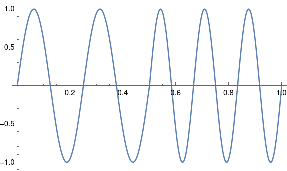
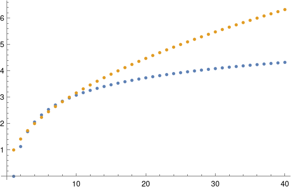
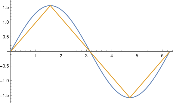
Even for a much larger declination of 60° = 1.047 radians, the two curves are fairly close together. The approximation, in blue, slightly overestimates the exact value, in gold.

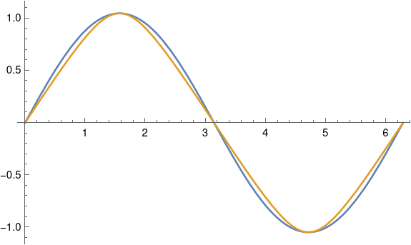
This plot was produced in Mathematica with

    ε = 60 Degree
    Plot[{ε Sin[θ] ], ArcSin[Sin[ε] Sin[θ]]}, {θ, 0, 2π}]

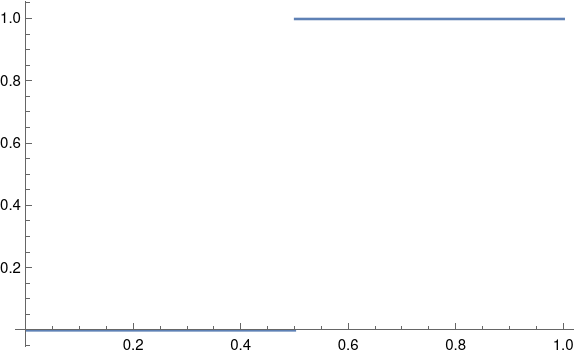
As ε gets larger, the curves start to separate. When ε = 90° the gold curve becomes exactly a triangular wave.

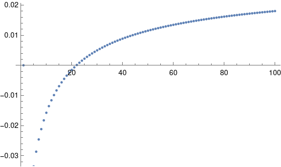
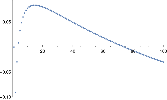
Update: Here’s a plot of the maximum approximation error as a function of ε.

Related posts

Reverse engineering Fourier conventions

The most annoying thing about Fourier analysis is that there are many slightly different definitions of the Fourier transform. One time I got sufficiently annoyed that I creates a sort of Rosetta Stone of Fourier theorems under eight different conventions. Later I discovered that Mathematica supports these same eight definitions, but with slightly different notation.

When I created my Rosetta Stone I wanted to have a set of notes that answered the question “What are the basic Fourier theorems under this convention?” Recently I was reading a reference and wanted to answer the opposite question “Given the theorems this book is stating, what convention must they be using?”

The eight definitions correspond to

\hat{f}(\omega) = \frac{1}{\sqrt{m}} \int_{-\infty}^\infty \exp(\sigma q i \omega x) f(x) \,dx

where m is either 1 or 2π, σ is +1 or −1, and q is 2π or 1.

I’m posting these notes for my future reference and for anyone else who may need to do the same sleuthing.

Notation

For the rest of the post, let F and G be the Fourier transforms of f and g respectively. We write

f(x) \leftrightarrow F(\omega)

for the pair of a function and its Fourier transform.

Define the inner product of f and g as

\langle f, g \rangle = \int_{-\infty}^\infty f(x)\, g(x) \, dx

if f and g are real-value. If the functions are complex-valued, replace g with the complex conjugate if g.

We will sometimes denote the Fourier transform of a function by putting a hat on top of it.

Convolution theorem

The convolution theorem gives a quick way to determine the parameter m. Suppose convolution is defined by

(f*g)(x) = \int_{-\infty}^\infty f(x-y)\, g(y) \, dy

Then

f(x)*g(x) \leftrightarrow \sqrt{m} F(\omega)*G(\omega)

and so you can find m immediately. If f*g = F*G with no extra factor out front, m = 1. Otherwise if there’s a factor of √2π out front, then m = 2π. If there’s any other factor, you’ve got an arcane definition of Fourier transform that isn’t one of the eight considered here.

Some authors, like Walter Rudin, include a scaling factor in the definition of convolution, in which casethe argument of this section doesn’t hold.

Parseval and Plancherel

Parseval’s theorem says that the inner product of f and g is proportional to the inner product of F and G. The proportionality constant depends on the definition of Fourier transform, specifically on m and q, and so you can determine m or q from the form of Parseval’s theorem.

\langle f, g \rangle = k \langle F, G \rangle

If k = 1, then either q = 2π and m = 1 or q = 1 and m = 2π. If you know m, say from the statement of the convolution theorem, then Parseval’s theorem tells you q.

Plancherel’s theorem is the special case of Parseval’s theorem with f = g. It can be used the same way to solve for m or q.

If k = 2π, then q = m = 1. If k= 1/2π, then q = m = 1.

Double transform

Theorems about taking the Fourier transform twice carry the same information as Parseval’s and Plancherel’s theorems, i.e. they also let you determine m or q.

We have

\hat{\hat{f}}(x) = k f(-x)

with the same conclusions based on k as above:

  • If k = 1, then either q = 2π and m = 1 or q = 1 and m = 2π.
  • If k = 2π, then q = m = 1.
  • If k= 1/2π, then q = m = 1.

Shift and differentiation

So far we none of our theorems have allowed us to reverse engineer σ. Either the shift or differentiation theorem will let is find σq.

The shift theorem says

f(x-h) \leftrightarrow \exp(ikh\omega) F(\omega)

where k = σq. Since σ = ±1 and q = 1 or 2π, the product σq determines both σ and q.

Similarly, the differentiation theorem says the Fourier transform of the derivative of f transforms as

f'(x) \leftrightarrow ik\omega F(\omega)

and again k = σq.

Dividing an octave into 14 pieces

Keenan Pepper left a comment on my previous post saying that the DTMF tones used by touch tone phones “are actually quite close to 14 equal divisions of the octave (rather than the usual 12).”

Let’s show that this is right using a little Python.

    import numpy as np

    freq = np.array([697, 770, 852, 941, 1209, 1336, 1477])
    lg = np.log2(freq)
    spacing = lg[1:] - lg[:-1]
    print(spacing)
    print([2/14, 2/14, 2/14, 5/14, 2/14, 2/14])

If the tones are evenly spaced on a 14-note scale, we’d expect the logarithms base 2 of the notes to differ by multiples of 1/14.

This produces the following:

    [0.144 0.146 0.143 0.362 0.144 0.145]
    [0.143 0.143 0.143 0.357 0.143 0.143]

By dividing the octave into 14 points the DFMT system largely avoids overlap between the set of tones and the set of their harmonics. However, the first overtone of the first tone (1394 Hz) is kinda close to the fundamental of the 6th tone (1336 Hz).

Plotting DTMF tones and first two harmonics

Related posts

Phone tones in musical notation

The sounds produced by a telephone keypad are a combination of two tones: one for the column and one for the row. This system is known as DTMF (dual tone multiple frequency).

I’ve long wondered what these tones would be in musical terms and I finally went to the effort to figure it out when I ran across DTMF in [1].

The three column frequencies are 1209, 1336, and 1477 Hz. These do not correspond exactly to standard musical pitches. The first frequency, 1209 Hz, is exactly between a D and a D#, two octaves above middle C. The second frequency, 1336 Hz, is 23 cents [2] higher than an E. The third frequency, 1477 Hz, lands on an F#.

In approximate musical notation, these pitches are two octaves above the ones written below.

Notice that the symbol in front of the D is a half sharp, one half of the symbol in front of the F.

Similarly, the four row frequencies, starting from the top, are 697, 770, 852, and 941 Hz. In musical terms, these notes are F, G (31 cents flat), A (54 cents flat), and B flat (16 cents sharp).


The backward flat symbol in front of the A is a half flat. As with the column frequencies, the row frequencies are two octaves higher than written.

These tones are deliberately not in traditional harmony because harmonic notes (in the musical sense) are harmonically related (in the Fourier analysis sense). The phone company wants tones that are easy to pull apart analytically.

Finally, here are the chords that correspond to each button on the phone keypad.

Update: Dial tone and busy signal

Related posts

[1] Electric Circuits by Nilsson and Riedel, 10th edition, page 548.
[2] A cent is 1/100 of a semitone.

Frequency shift keying (FSK) spectrum

This post will look encoding digital data as an analog signal using frequency shift keying (FSK), first directly and then with windowing. We’ll look at the spectrum of the encoded signal and show that basic FSK uses much less bandwidth than direct encoding, but more bandwidth than FSK with windowing.

Square waves

The most natural way to encode binary data as an analog signal would be represent 0s and 1s by a sequence of pulses that take on the values 0 and 1.

A problem with this approach is that it would require a lot of bandwidth.

In theory a square wave has infinite bandwidth: its Fourier series has an infinite number of non-zero coefficients. In practice, the bandwidth of a signal is determined by how many Fourier coefficients it has above some threshold. The threshold would depend on context, but let’s say we ignore Fourier components with amplitude smaller than 0.001.

As I wrote about here, the nth Fourier sine series coefficients for a square wave is equal to 4/nπ for odd n. This means we would need on the order of 1,000 terms before the coefficients drop below our threshold.

Frequency shift keying

The rate of convergence of the Fourier series for a function f depends on the smoothness of f. Discontinuities, like the jump in a square wave, correspond to slow convergence, i.e. high bandwidth. We can save bandwidth by encoding our data with smoother functions.

So instead of jumping from 0 to 1, we’ll encode a 0 as a signal of one frequency and a 1 as a signal with another frequency. By changing the frequency after some whole number of periods, the resulting function will be continuous, and so will have smaller bandwidth.

Suppose we have a one second signal f(t) that is made of half a second of a 4 Hz signal and half a second of a 6 Hz signal, possibly encoding a 0 followed by a 1.

What would the Fourier coefficients look like? If we just had a 4 Hz sine wave, the Fourier series would have only one component: the signal itself at 4 Hz. If we just had a 6 Hz sine wave, the only Fourier component would again be the signal itself. There would be no sine components at other frequencies, and no cosine components.

But our signal patched together by concatenating 4 Hz and 6 Hz signals has non-zero cosine terms for every odd n, and these coefficients decay like O(1/n²).

Our Fourier series is

f(t) = 0.25 sin 8πt + 0.25 sin 12πt + 0.0303 cos 2πt + 0.1112 cos 6πt − 0.3151 cos 12πt + 0.1083 cos 10πt + …

We need to go out to 141 Hz before the coefficients drop below 0.001. That’s a lot of coefficients, but it’s an order of magnitude fewer coefficients than we’d need for a square wave.

Pulse shaping

Although our function f is continuous, it is not differentiable. The left-hand derivative at 1/2 is 8π and the right-hand derivative is 12π. If we could replace f with a related function that is differentiable at 1/2, presumably the signal would require less bandwidth.

We could do this by multiplying both halves of our signal by a windowing function. This is called pulse shaping because instead of a simple sine wave, we change the shape of the wave, tapering it at the ends.

Let’s using a cosine window because that’ll be easy; in practice you’d probably use a different window [1].

Now our function is differentiable at 1/2, and its Fourier series converges more quickly. Now we can disregard components above 40 Hz. With a smoother windowing function the windowed function would have more derivatives and we could disregard more of the high frequencies.

Related posts

[1] This kind of window is called a cosine window because you multiply your signal by one lobe of a cosine function, with the peak in the middle of the signal. Since we’re doing this over [0. 1/2] and again over [1/2, 1], we’re actually multiplying by |sin 2πt|.

Approximating the range of normal samples

On Monday I wrote a blog post that showed you can estimate the standard deviation of a set of data by first computing its range and then multiplying by a constant. The advantage is that it’s easy to compute a range, but computing a standard deviation in your head would be tedious to say the least.

The problem, or the interesting part, depending on your perspective, is the constants dn you have to multiply the range by.

Yesterday before work I wrote a blog post about a proposed approximation dn and yesterday after work I wrote a post on the exact values.

There have been a couple suggestions in the comments for how to approximate dn, namely √n and log n. There’s merit to both over different ranges.

Here’s a plot of dn and √n. You can see that √n is an excellent approximation to dn for n between 3 and 10: the gold and blue dots overlap. But for larger n, √n grows too fast. It keeps going while dn sorta plateaus.

For larger n, log n is a better approximation to dn. When n = 100, the square root approximation is about twice the exact value, but the log approximation if fairly close. The error in the log approximation seems to be decreasing slowly, maybe going to zero or to a small constant.

There are more accurate approximations out there. In 1958, Gunnar Blom [1] published the approximation

E(r, n) = - \Phi^{-1}\left( \frac{r - \alpha}{n - 2\alpha + 1} \right)

You can get good results for moderately large n by taking α = 0.375, and you can get even better results by adjusting α over various ranges of r and n.

As I wrote last night, E(r, n) is the expected value of the rth order statistic from a sample of size n, Φ is the CDF of a standard normal, and dn = 2 E(n, n).

We can implement Blom’s approximation with the following Mathematica code.

    PhiInv[x_] := Sqrt[2] InverseErf[2 x - 1]
    alpha = 0.375
    Blom[n_] := -2 PhiInv[(1 - alpha)/(n - 2 alpha + 1)]

If we plot dn and Blom’s approximation on the same plot, we won’t be able to tell them apart: the dots overlap. We can plot the difference between the two values with

    ListPlot[Table[d[n] - Blom[n], {n, 1, 100}]]

and get the following graph.

There have been more accurate approximations developed since 1958, but that’s as far as I want to go down this rabbit hole for now.

Update: I just noticed a comment on the first post in this series. Ashley Kanter’s approximation was supposed to be

3 (log10 n) 0.75

and not

3 log10 (n0.75)

The former is quite good, with a an error comparable to Blom’s method. Here’s a plot of the error:


[1] Gunnar Blom (1958). Statistical Estimates and Transformed Beta-Variables. John Wiley and Sons Inc.

Order statistics for normal distributions

The last couple posts have touched on order statistics for normal random variables. I wrote the posts quickly and didn’t go into much detail, and more detail would be useful.

Given two integers nr ≥ 1, define E(r, n) to be the rth order statistic of n samples from standard normal random variables. That is, if we were to take n samples and then sort them in increasing order, the expected value of the rth sample is E(r, n).

We can compute E(r, n) exactly by

E(r, n) = \frac{n!}{(r-1)!\, (n-r)!} \int_{-\infty}^\infty x (1 - \Phi(x))^{r-1}\,\Phi(x)^{n-r}\, \phi(x) \, dx

where φ and Φ are the PDF and CDF of a standard normal random variable respectively. We can numerically evaluate E(r, n) by numerically evaluating its defining integral.

The previous posts have used

dn = E(n, n) – E(1, n) = 2 E(n, n).

The second equality above follows by symmetry.

We can compute dn in Mathematica as follows.

    Phi[x_] := (1 + Erf[x/Sqrt[2]])/2    
    phi[x_] := Exp[-x^2/2]/Sqrt[2 Pi]
    d[n_] := 2 n NIntegrate[
        x Phi[x]^(n - 1) phi[x], {x, -Infinity, Infinity}]

And we can reproduce the table here by

    Table[1/d[n], {n, 2, 10}]

Finally, we can see how dn behaves for large n by calling

    ListPlot[Table[d[n], {n, 1, 1000}]]

to produce the following graph.

See the next post for approximations to dn.

Range trick for larger sample sizes

The previous post showed that the standard deviation of a sample of size n can be well estimated by multiplying the sample range by a constant dn that depends on n.

The method works well for relatively small n. This should sound strange: typically statistical methods work better for large samples, not small samples. And indeed this method would work better for larger samples. However, we’re not so much interested in the efficiency of the method per se, but its efficiency relative to the standard way of estimating standard deviation. For small samples, both methods are not very accurate, and the two methods appear to work equally well.

If we want to use the range method for larger n, there are a couple questions: how well does the method work, and how do we calculate dn.

Simple extension

Ashley Kanter left a comment on the previous post saying

dn = 3 log n0.75 (where the log is base 10) seems to perform quite well even for larger n.

Ashley doesn’t say where this came from. Maybe it’s an empirical fit.

The constant dn is the expected value of the range of n samples from a standard normal random variable. You could find a (complicated) expression for this and then find a simpler expression using an asymptotic approximation. Maybe I’ll try that later, but for now I need to wrap up this post and move on to client work.

Note that

log10 n0.75 = 0.977 loge(n)

and so we could use

dn = log n

where log is natural log. This seems like something that might fall out of an asymptotic approximation. Maybe Ashley empirically discovered the first term of a series approximation.

Update: See this post for a more detailed exploration of how well log n, square root of n, and another method approximate dn.

Update 2: Ashley Kanter’s approximation was supposed to be 3 (log10 n) 0.75 rather than 3 log10 (n0.75) and is a very good approximation. This is also addressed in the link in the first update.

Simulation

Here’s some Python code to try things out.

    import numpy as np
    from scipy.stats import norm

    np.random.seed(20220309)

    n = 20
    for _ in range(5):
        x = norm.rvs(size=n)
        w = x.max() - x.min()
        print(x.std(ddof=1), w/np.log(n))

And here are the results.

    |   std | w/d_n |
    |-------+-------|
    | 0.930 | 1.340 |
    | 0.919 | 1.104 |
    | 0.999 | 1.270 |
    | 0.735 | 0.963 |
    | 0.956 | 1.175 |

It seems the range method has more variance, though notice in the fourth row that the standard estimate can occasionally wander pretty far from the theoretical value of 1 as well.

We get similar results when we increase n to 50.

    |   std | w/d_n |
    |-------+-------|
    | 0.926 | 1.077 |
    | 0.889 | 1.001 |
    | 0.982 | 1.276 |
    | 1.038 | 1.340 |
    | 1.025 | 1.209 |

Not-so-simple extension

There are ways to improve the range method, if by “improve” you mean make it more accurate. One way is to divide the sample into random partitions, apply the method to each partition, and average the results. If you’re going to do this, partitions of size 8 are optimal [1]. However, the main benefit of the range method [2] is its simplicity.

Related posts

[1] F. E. Grubbs and C. L. Weaver (1947). The best unbiased estimate of a population standard deviation based on group ranges. Journal of the American Statistical Association 42, pp 224–41

[2] The main advantage now is its simplicity, When it was discovered, the method reduced manual calculation, and so it could have been worthwhile to make the method a little more complicated as long as the calculation effort was still less than that of the standard method.

Estimating standard deviation from range

Suppose you have a small number of samples, say between 2 and 10, and you’d like to estimate the standard deviation σ of the population these samples came from. Of course you could compute the sample standard deviation, but there is a simple and robust alternative.

Let W be the range of our samples, the difference between the largest and smallest value. Think “w” for “width.” Then

W / dn

is an unbiased estimator of σ where the constants dn can be looked up in a table [1].

    |  n | 1/d_n |
    |----+-------|
    |  2 | 0.886 |
    |  3 | 0.591 |
    |  4 | 0.486 |
    |  5 | 0.430 |
    |  6 | 0.395 |
    |  7 | 0.370 |
    |  8 | 0.351 |
    |  9 | 0.337 |
    | 10 | 0.325 |

The values dn in the table were calculated from the expected value of W/σ for normal random variables, but the method may be used on data that do not come from a normal distribution.

Let’s try this out with a little Python code. First we’ll take samples from a standard normal distribution, so the population standard deviation is 1. We’ll draw five samples, and estimate the standard deviation two ways: by the method above and by the sample standard deviation.

    from scipy.stats import norm, gamma

    for _ in range(5):
        x = norm.rvs(size=10)
        w = x.max() - x.min()
        print(x.std(ddof=1), w*0.325)

Here’s the output:

    | w/d_n |   std |
    |-------+-------|
    | 1.174 | 1.434 |
    | 1.205 | 1.480 |
    | 1.173 | 0.987 |
    | 1.154 | 1.277 |
    | 0.921 | 1.083 |

Just from this example it seems the range method does about as well as the sample standard deviation.

For a non-normal example, let’s repeat our exercise using a gamma distribution with shape 4, which has standard deviation 2.

    | w/d_n |   std |
    |-------+-------|
    | 2.009 | 1.827 |
    | 1.474 | 1.416 |
    | 1.898 | 2.032 |
    | 2.346 | 2.252 |
    | 2.566 | 2.213 |

Once again, it seems both methods do about equally well. In both examples the uncertainty due to the small sample size is more important than the difference between the two methods.

Update: To calculate dn for other values of n, see this post.

[1] Source: H, A. David. Order Statistics. John Wiley and Sons, 1970.

Varicode

Varicode is a way of encoding text and control characters into binary using code words of variable length. It was developed as part of the PSK31 protocol for digital communication over amateur radio.

In the spirit of Morse code, it uses short code words for common characters and longer code words for less common characters in the expectation that this will result in shorter encodings.

If you use variable length words, you’ve got to have some way of knowing when one word ends and the next begins. Varicode solves this problem by using only keywords that begin and end with 1 and that do not contain two consecutive zeros. Then 00 is inserted between code words. Since 00 cannot appear inside a code word, these bits unambiguously mark the space between code words.

Synchronization

Varicode is self-synchronizing in the sense that if you jump into a stream of bits produced by Varicode, as soon as you see two zeros, you know you’re at a code word boundary and can start reading from there. You’ve lost any bits that were transmitted before you jumped in, but you can parse everything going forward.

ASCII doesn’t have this problem or this robustness. It doesn’t have the problem of determining code word boundaries because every code word is eight bits long. But then to read a stream of ASCII bits you need to know your position mod 8. If you jump into a stream of bits, you don’t know where the next code word boundary will be, though you may be able to infer it by trying 8 possibilities and seeing which produces the most intelligible results.

Regular expression

Another way to state the rules for forming Varicode code words is to say that 1 is a valid code (the code for a space, ASCII 0x20) and that you can form new codes by prefixing 1 or 10 to a code. In terms of regular expressions, this says a Varicode code word matches

    (1|10)*1

Fibonacci numbers

How many code words are there of length n? Well, there are two ways to make a code word that long: you either put a 1 in front of a code word of length n-1, or you put a 10 in front of a code word of length n-2. So the number of code words of length n equals the number of code words of length n-1 plus the number of code words of length n-2. That is, the number of code words satisfies the same recurrence relation as the Fibonacci numbers.

It’s easy to see that there’s only one code word of length one, and only one code word of length two, so the number of code words of each length satisfies the initial conditions for the Fibonacci sequence as well, and so they are the Fibonacci numbers.

Efficiency

Varicode encodes a lot more than lower case letters—it encodes most ASCII characters— and so it would take some work to discover the relative frequencies of the characters, and this frequency would depend on where Varicode is used. As far as I know Varicode is use primarily (only?) in PSK31, and so the relevant frequency would be the frequencies in messages sent over PSK31, not English more generally.

You can find the code words of each letter here.

To make things easier, let’s suppose messages are limited to lower case letters and spaces, and that the letters follow the same distribution as in English in general.

We can use the letter frequencies here, except these don’t take spaces into account. If we assume words are about 5 letters long, then the probability of a character being a space is 1/6 and the probabilities of the other characters conditional on not being a space are given by the table. This means the letter probabilities need to be multiplied by 5/6.

This gives us a an expected length of 3.89 bits per letter, which is effectively 5.89 bits when you consider the 00 pattern we have to add between letters.

You could represent the 26 letters and a few more characters using 5 bits, but the result would not be self-synchronizing. One way of looking at this to say that the compression provided by variable length encoding nearly pays for the overhead required to make the code self-synchronizing.

Related posts