I try to maintain a consistent work environment across computers that I use. The computers differ for important reasons, but I’d rather they not differ for unimportant reasons.
Unified keys
One thing I do is remap keys so that the same key does the same thing everywhere, to the extent that’s practical. This requires remapping keys. In particular, I want the key functionality, not the key name, to be the same across operating systems. For example, the Command key on a Mac does what the Control key does on Windows and Linux. I have my machines set up so the key in the lower left corner, whatever you call it, does things like copy, paste, and cut.
Unified config files
I use bash everywhere even though zshell is the default on Mac OS. But Linux and MacOS are sufficiently different that I have two .bashrc files, one for each OS. However, both .bashrc files source a common file .bash_aliases for aliases. You can set that up by putting the following code in your .bashrc file.
if [ -f ~/.bash_aliases ]; then
    . ~/.bash_aliases
fi
Sometimes you need some kind of branching logic even for two machines running the same OS. For example, if you have two computers, named Castor and Pollux, you might have code like the following in your .bashrc.
HOSTNAME_SHORT=$(hostname -s)
if [ "$HOSTNAME_SHORT" = "Castor" ]; then
...
elif [ "$HOSTNAME_SHORT" = "Pollux" ]; then
...
One problem with using hostname is that the OS can change the name on you. At least MacOS will do this; I don’t know whether other operating systems will. If you give your machine an uncommon name then this is unlikely to happen.
I have one init.el file for Emacs. It contains some branching logic for OS:
(cond
    ((string-equal system-type "windows-nt") ; Microsoft Windows
     ...)
    ((string-equal system-type "gnu/linux") ; linux
     ...)
    ((string-equal system-type "darwin") ; Mac
     ...)
)
You can also branch on hostname.
(if (string-equal (system-name) "Castor")
...)
(if (string-equal (system-name) "Pollux")
...)
This isn’t difficult, but in the short run it’s easier to just make one ad hoc edit to a config file at a time, letting the files drift apart. Along those lines, see bicycle skills.

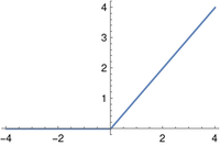
![\partial f(x) = \left\{ \begin{array}{cl} 1 & \text{if } x > 0 \\<br /> \left[0,1\right] & \text{if } x = 0 \\<br /> 0 & \text{if } x < 0 \end{array} \right.](https://www.johndcook.com/subgradient.svg)


![\left(\frac{g}{h}\right)^{(n)} = \frac{1}{h^{\,n+1}} \left| \begin{array}{cccccc} h & 0 & 0 & \cdots & 0 & g \\[3pt] h^\prime & h & 0 & \cdots & 0 & g^\prime \\[3pt] h^{\prime\prime} & 2h^\prime & h & \cdots & 0 & g^{\prime\prime} \\[3pt] \cdots & \cdots & \cdots & \cdots & \cdots & \cdots \\[3pt] h^{(n)} & \binom{n}{1}h^{(n-1)} & \binom{n}{2}h^{(n-2)} & \cdots & \binom{n}{1}h^\prime & g^{(n)} \end{array} \right|](https://www.johndcook.com/quotientn.svg)