Computing SVD and pseudoinverse

In a nutshell, given the singular decomposition of a matrix A,

A = U \Sigma V^*

the Moore-Penrose pseudoinverse is given by

A^+ = V \Sigma^+ U^*.

This post will explain what the terms above mean, and how to compute them in Python and in Mathematica.

Singular Value Decomposition (SVD)

The singular value decomposition of a matrix is a sort of change of coordinates that makes the matrix simple, a generalization of diagonalization.

Matrix diagonalization

If a square matrix A is diagonalizable, then there is a matrix P such that

A = P D P^{-1}

where the matrix D is diagonal. You could think of P as a change of coordinates that makes the action of A as simple as possible. The elements on the diagonal of D are the eigenvalues of A and the columns of P are the corresponding eigenvectors.

Unfortunately not all matrices can be diagonalized. Singular value decomposition is a way to do something like diagonalization for any matrix, even non-square matrices.

Generalization to SVD

Singular value decomposition generalizes diagonalization. The matrix Σ in SVD is analogous to D in diagonalization. Σ is diagonal, though it may not be square. The matrices on either side of Σ are analogous to the matrix P in diagonalization, though now there are two different matrices, and they are not necessarily inverses of each other. The matrices U and V are square, but not necessarily of the same dimension.

The elements along the diagonal of Σ are not necessarily eigenvalues but singular values, which are a generalization of eigenvalues. Similarly the columns of U and V are not necessarily eigenvectors but left singular vectors and right singular vectors respectively.

The star superscript indicates conjugate transpose. If a matrix has all real components, then the conjugate transpose is just the transpose. But if the matrix has complex entries, you take the conjugate and transpose each entry.

The matrices U and V are unitary. A matrix M is unitary if its inverse is its conjugate transpose, i.e. M* M = MM* = I.

Pseudoinverse and SVD

The (Moore-Penrose) pseudoinverse of a matrix generalizes the notion of an inverse, somewhat like the way SVD generalized diagonalization. Not every matrix has an inverse, but every matrix has a pseudoinverse, even non-square matrices.

Computing the pseudoinverse from the SVD is simple.

If

A = U \Sigma V^*

then

A^+ = V \Sigma^+ U^*

where Σ+ is formed from Σ by taking the reciprocal of all the non-zero elements, leaving all the zeros alone, and making the matrix the right shape: if Σ is an m by n matrix, then Σ+ must be an n by m matrix.

We’ll give examples below in Mathematica and Python.

Computing SVD in Mathematica

Let’s start with the matrix A below.

A = \begin{bmatrix} 2 & -1 & 0 \\ 4 & 3 & -2 \end{bmatrix}

We can find the SVD of A with the following Mathematica commands.

    A = {{2, -1, 0}, {4, 3, -2}}
    {U, S, V} = SingularValueDecomposition[A]

From this we learn that the singular value decomposition of A is

\begin{bmatrix} \frac{1}{\sqrt{26}} & -\frac{5}{\sqrt{26}} \\ \frac{5}{\sqrt{26}} & \frac{1}{\sqrt{26}} \\ \end{bmatrix} \begin{bmatrix} \sqrt{30} & 0 & 0 \\ 0 & 2 & 0 \end{bmatrix} \begin{bmatrix} \frac{11}{\sqrt{195}} & \frac{7}{\sqrt{195}} & -\sqrt{\frac{5}{39}} \\ -\frac{3}{\sqrt{26}} & 2 \sqrt{\frac{2}{13}} & -\frac{1}{\sqrt{26}} \\ \frac{1}{\sqrt{30}} & \sqrt{\frac{2}{15}} & \sqrt{\frac{5}{6}} \end{bmatrix}

Note that the last matrix is not V but the transpose of V. Mathematica returns V itself, not its transpose.

If we multiply the matrices back together we can verify that we get A back.

    U . S. Transpose[V]

This returns

    {{2, -1, 0}, {4, 3, -2}}

as we’d expect.

Computing pseudoinverse in Mathematica

The Mathematica command for computing the pseudoinverse is simply PseudoInverse. (The best thing about Mathematica is it’s consistent, predictable naming.)

    PseudoInverse[A]

This returns

    {{19/60, 1/12}, {-(11/30), 1/6}, {1/12, -(1/12)}}

And we can confirm that computing the pseudoinverse via the SVD

    Sp = {{1/Sqrt[30], 0}, {0, 1/2}, {0, 0}}
    V . Sp . Transpose[U]

gives the same result.

Computing SVD in Python

Next we compute the singular value decomposition in Python (NumPy).

    >>> a = np.matrix([[2, -1, 0],[4,3,-2]])
    >>> u, s, vt = np.linalg.svd(a, full_matrices=True)

Note that np.linalg.svd returns the transpose of V, not the V in the definition of singular value decomposition.

Also, the object s is not the diagonal matrix Σ but a vector containing only the diagonal elements, i.e. just the singular values. This can save a lot of space if the matrix is large. The NumPy method svd has other efficiency-related options that I won’t go into here.

We can verify that the SVD is correct by turning s back into a matrix and multiply the components together.

    >>> ss = np.matrix([[s[0], 0, 0], [0, s[1], 0]])
    >>> u*ss*vt

This returns the matrix A, within floating point accuracy. Since Python is doing floating point computations, not symbolic calculation like Mathematica, the zero in A turns into -3.8e-16.

Note that the singular value decompositions as computed by Mathematica and Python differ in a few signs here and there; the SVD is not unique.

Computing pseudoinverse in Python

The pseudoinverse can be computed in NumPy with np.linalg.pinv.

    >>> np.linalg.pinv(a)
    matrix([[ 0.31666667,  0.08333333],
            [-0.36666667,  0.16666667],
            [ 0.08333333, -0.08333333]])

This returns the same result as Mathematica above, up to floating point precision.

More linear algebra posts

Probability of coprime sets

The latest blog post from Gödel’s Lost Letter and P=NP looks at the problem of finding relatively prime pairs of large numbers. In particular, they want a deterministic algorithm. They mention in passing that the probability of a set of k large integers being relatively prime (coprime) is 1/ζ(k) where ζ is the Riemann zeta function. This blog post will look closer at that statement.

How large is large?

What does it mean that the numbers are large? That they are large enough that the asymptotic result given by the zeta function is accurate enough. We’ll explore this with simulation code shortly.

The exact statement is that in the limit as N goes to infinity, the probability of k integers chosen uniformly from 1 to N being coprime converges to 1/ζ(k). I won’t go into the proof here, but in a nutshell, it falls out of Euler’s product formula for the zeta function.

What does it mean for a set of numbers to be coprime?

The probability above seemed wrong to me at first. The function ζ(k) decreases as k increases, and so its reciprocal increases. That means it’s more likely that a set of numbers is coprime as the size of the set increases. But the larger the set of numbers, the more likely it is that two will have a common factor, so shouldn’t the probability that they’re coprime go down with k, not up?

The resolution to the apparent contradiction is that I had the wrong idea of coprime in mind. Two integers are coprime if they have no prime factors in common. How do you generalize that to more than two integers? You could define a set of numbers to be coprime if every pair of numbers in the set is coprime. That’s the definition I had in mind. But that’s not the standard definition. The right definition here is that the greatest common divisor of the set is 1. For example, (6, 14, 21) would be coprime because no single prime divides all three numbers, even though no pair of numbers from the set is coprime.

Python simulation

Let’s write some Python code to try this out. We’ll randomly generate some sets of large numbers and see how often they’re coprime.

How do you generate large random integers in Python? You can use the function getrandbits to generate numbers as large as you like. In the code below we’ll generate 128-bit integers.

How do you compute the greatest common divisor in Python? There’s a library function gcd, but it only takes two integers. We’ll use the reduce function to fold gcd over a list of integers.

How do you compute the zeta function in Python? SciPy doesn’t have an implementation of ζ(x) per se, but it does have an implementation of ζ(x)-1. Why not just implement ζ itself? Because for large x, ζ(x) is close to 1, so more precision can be saved by computing ζ − 1.

Putting these pieces together, here’s code to randomly generate triples of 128-bit integers, see how often they’re coprime, and compare the result to 1/ζ(3).

    from random import getrandbits
    from fractions import gcd
    from functools import reduce
    from scipy.special import zetac
    
    def riemann_zeta(x):
        return zetac(x) + 1
    
    k = 3
    size = 128
    N = 10000
    
    coprime_count = 0
    for _ in range(N):
        x = [getrandbits(size) for _ in range(k)]
        if reduce(gcd, x) == 1:
            coprime_count += 1
    print(coprime_count/N)
    print(1/riemann_zeta(k))

When I ran this I got

    0.8363
    0.831907372581

Simulation agrees with theory to two decimal places, which is just what we should expect from 10,000 repetitions. (We’d expect error on the order of 1/√N.)

Here’s what I got when I changed k to 4:

    0.9234
    0.923938402922

And here’s what I got for k set to 5:

    0.9632
    0.964387340429

Related posts

Obesity index: Measuring the fatness of probability distribution tails

A probability distribution is called “fat tailed” if its probability density goes to zero slowly. Slowly relative to what? That is often implicit and left up to context, but generally speaking the exponential distribution is the dividing line. Probability densities that decay faster than the exponential distribution are called “thin” or “light,” and densities that decay slower are called “thick”, “heavy,” or “fat,” or more technically “subexponential.” The distinction is important because fat-tailed distributions tend to defy our intuition.

One surprising property of heavy-tailed (subexponential) distributions is the single big jump principle. Roughly speaking, most of the contribution to the sum of several heavy-tailed random variables comes from the largest of the samples. To be more specific, let “several” = 4 for reasons that’ll be apparent soon, though the result is true for any n. As x goes to infinity, the probability that

X1 + X2 + X3 + X4

is larger than a given x is asymptotically equal the probability that

max(X1, X2, X3, X4)

is larger than the same x.

The idea behind the obesity index [1] is to turn the theorem above around, making it an empirical measure of how thick a distribution’s tail is. If you draw four samples from a random variable and sort them, the obesity index is the probability that that the sum of the max and min, X1 + X4, is greater than the sum of the middle samples, X2 + X3.

The obesity index could be defined for any distribution, but it only measures what the name implies for right-tailed distributions. For any symmetric distribution, the obesity index is exactly 1/2. A Cauchy distribution is heavy-tailed, but it has two equally heavy tails, and so its obesity index is the same as the normal distribution, which has two light tails.

Note that location and scale parameters have no effect on the obesity index; shifting and scaling effect all the X values the same, so it doesn’t change the probability that X1 + X4 is greater than X2 + X3.

To get an idea of the obesity index in action, we’ll look at the normal, exponential, and Cauchy distributions, since these are the canonical examples of thin, medium, and thick tailed distributions. But for reasons explained above, we’ll actually look at the folded normal and folded Cauchy distributions, i.e. we’ll take their absolute values to create right-tailed distributions.

To calculate the obesity index exactly you’d need to do analytical calculations with order statistics. We’ll simulate the obesity index because that’s easier. It’s also more in the spirit of calculating the obesity index from data.

    from scipy.stats import norm, expon, cauchy

    def simulate_obesity(dist, N):
        data = abs(dist.rvs(size=(N,4)))
        count = 0
        for row in range(N):
            X = sorted(data[row])
            if X[0] + X[3] > X[1] + X[2]:
                count += 1
        return count/N

    for dist in [norm, expon, cauchy]:
        print( simulate_obesity(dist, 10000) )

When I ran the Python code above, I got

    0.6692
    0.7519
    0.8396

This ranks the three distributions in the anticipated order of tail thickness.

Note that the code above takes the absolute value of the random samples. This lets us pass in ordinary (unfolded) versions of the normal and Cauchy distributions, and its redundant for any distribution like the exponential that’s already positive-valued.

[I found out after writing this blog post that SciPy now has foldnorm and foldcauchy, but they don’t seem to work like I expect.]

Let’s try it on a few more distributions. Lognormal is between exponential and Cauchy in thickness. A Pareto distribution with parameter b goes to zero like x−1−b and so we expect a Pareto distribution to have a smaller obesity index than Cauchy when b is greater than 1, and a larger index when b is less than one. Once again the simulation results are what we’d expect.

The code

    for dist in [lognorm, pareto(2), pareto(0.5)]:
        print( simulate_obesity(dist, 10000) )

returns

    0.7766
    0.8242
    0.9249

By this measure, lognormal is just a little heavier than exponential. Pareto(2) comes in lighter than Cauchy, but not by much, and Pareto(0.5) comes in heavier.

Since the obesity index is a probability, it will always return a value between 0 and 1. Maybe it would be easier to interpret if we did something like take the logit transform of the index to spread the values out more. Then the distinctions between Pareto distributions of different orders, for example, might match intuition better.

[1] Roger M. Cooke et al. Fat-Tailed Distributions: Data, Diagnostics and Dependence. Wiley, 2014.

Squared digit sum

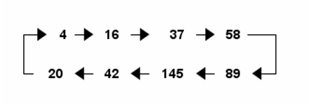
Take any positive integer n and sum the squares of its digits. If you repeat this operation, eventually you’ll either end at 1 or cycle between the eight values 4, 16, 37, 58, 89, 145, 42, and 20.

For example, pick n = 389. Then 3² + 8² + 9² = 9 + 64 + 81 = 154.

Next, 1² + 5² + 4² = 1 + 25 + 16 = 42, and now we’re at one of the eight special values. You can easily verify that once you land on one of these values you keep cycling.

The following code shows that the claim above is true for numbers up to 1,000.

    def square_digits(n):
        return sum( int(c)**2 for c in str(n) )

    attractors = [1, 4, 16, 37, 58, 89, 145, 42, 20]

    for n in range(1, 1000):
        m = n
        while m not in attractors:
            m = square_digits(m)

    print("Done")

For a proof that the claim is true in general, see “A Set of Eight Numbers” by Arthur Porges, The American Mathematical Monthly, Vol. 52, No. 7, pp. 379-382.

***

By the way, the cycle image above was created with Emacs org-mode using the following code.

    #+BEGIN_SRC ditaa :file square_digit_sum_cycle.png

    +-> 4 -> 16 ->  37 -> 58---+
    |                          |
    |                          |
    +- 20 <- 42 <- 145 <- 89 <-+     

    #+END_SRC

It’s not the prettiest output, but it was quick to produce. More on producing ASCII art graphs here.

Equation for the Eiffel Tower

Robert Banks’s book Towing Icebergs, Falling Dominoes, and Other Adventures in Applied Mathematics describes the Eiffel Tower’s shape as approximately the logarithmic curve

y = -y_* \log\left(\frac{x}{x_0} \right )

where y* and x0 are chosen to match the tower’s dimensions.

Here’s a plot of the curve:

Eiffel tower curve plot

And here’s the code that produced the plot:

from numpy import log, exp, linspace, vectorize
import matplotlib.pyplot as plt

# Taken from "Towing Icebergs, Falling Dominoes,
# and Other Adventures in Applied Mathematics"
# by Robert B. Banks

# Constants given in Banks in feet. Convert to meters.
feet_to_meter = 0.0254*12
ystar  = 201*feet_to_meter
x0     = 207*feet_to_meter
height = 984*feet_to_meter

# Solve for where to cut off curve to match height of the tower.
# - ystar log xmin/x0 = height
xmin = x0 * exp(-height/ystar)

def f(x):
    if -xmin < x < xmin:
        return height
    else:
        return -ystar*log(abs(x/x0))
curve = vectorize(f)
    
x = linspace(-x0, x0, 400)

plt.plot(x, curve(x))
plt.xlim(-2*x0, 2*x0)
plt.xlabel("Meters")
plt.ylabel("Meters")
plt.title("Eiffel Tower")

plt.axes().set_aspect(1)
plt.savefig("eiffel_tower.svg")

Related post: When length equals area
The St. Louis arch is approximately a catenary, i.e. a hyperbolic cosine.

Fourier-Bessel series and Gibbs phenomena

Fourier-Bessel series are analogous to Fourier series. And like Fourier series, they converge pointwise near a discontinuity with the same kind of overshoot and undershoot known as the Gibbs phenomenon.

Fourier-Bessel series

Bessel functions come up naturally when working in polar coordinates, just as sines and cosines come up naturally when working in rectangular coordinates. You can think of Bessel functions as a sort of variation on sine waves. Or even more accurately, a variation on sinc functions, where sinc(z) = sin(z)/z. [1]

A Fourier series represents a function as a sum of sines and cosines of different frequencies. To make things a little simpler here, I’ll only consider Fourier sine series so I don’t have to repeatedly say “and cosine.”

f(z) = \sum_{n=1}^\infty c_n \sin(n \pi z)

A Fourier-Bessel function does something similar. It represents a function as a sum of rescaled versions of a particular Bessel function. We’ll use the Bessel J0 here, but you could pick some other Jν.

Fourier series scale the sine and cosine functions by π times integers, i.e. sin(πz), sin(2πz), sin(3πz), etc. Fourier-Bessel series scale by the zeros of the Bessel function: J01z),  J02z),  J03z), etc. where λn are the zeros of J0. This is analogous to scaling sin(πz) by its roots: π, 2π, 3π, etc. So a Fourier-Bessel series for a function f looks like

f(z) = \sum_{n=1}^\infty c_n J_0(\lambda_n z).

The coefficients cn for Fourier-Bessel series can be computed analogously to Fourier coefficients, but with a couple minor complications. First, the basis functions of a Fourier series are orthogonal over [0, 1] without any explicit weight, i.e. with weight 1. And second, the inner product of a basis function doesn’t depend on the frequency. In detail,

\int_0^1 \sin(m \pi z) \, \sin(n \pi z) \, dz = \frac{\delta_{mn}}{2}.

Here δmn equals 1 if m = n and 0 otherwise.

Fourier-Bessel basis functions are orthogonal with a weight z, and the inner product of a basis function with itself depends on the frequency. In detail

\int_0^1 J_0(\lambda_m z) \, J_0(\lambda_n z) \, z\, dz = \frac{\delta_{mn}}{2} J_1(\lambda_n).

So whereas the coefficients for a Fourier sine series are given by

c_n = 2 \int_0^1 f(z)\, \sin(n\pi z) \,dz

the coefficients for a Fourier-Bessel series are given by

c_n = \frac{ 2\int_0^1 f(z)\, J_0(\lambda_n z) \, dz}{ J_1(\lambda_n)^2 }.

Gibbs phenomenon

Fourier and Fourier-Bessel series are examples of orthogonal series, and so by construction they converge in the norm given by their associated inner product. That means that if SN is the Nth partial sum of a Fourier series

\lim_{N\to\infty} \int_0^1 \left( f(x) - S_N(x) \right)^2 \, dz = 0
and the analogous statement for a Fourier-Bessel series is

\lim_{N\to\infty} \int_0^1 \left( f(x) - S_N(x) \right)^2 \, z\, dz = 0.

In short, the series converge in a (weighted) L² norm. But how do the series converge pointwise? A lot of harmonic analysis is devoted to answering this question, what conditions on the function f guarantee what kind of behavior of the partial sums of the series expansion.

If we look at the Fourier series for a step function, the partial sums converge pointwise everywhere except at the step discontinuity. But the way they converge is interesting. You get a sort of “bat ear” phenomena where the partial sums overshoot the step function at the discontinuity. This is called the Gibbs phenomenon after Josiah Willard Gibbs who observed the effect in 1899. (Henry Wilbraham observed the same thing earlier, but Gibbs didn’t know that.)

The Gibbs phenomena is well known for Fourier series. It’s not as well known that the same phenomenon occurs for other orthogonal series, such as Fourier-Bessel series. I’ll give an example of Gibbs phenomenon for Fourier-Bessel series taken from [2] and give Python code to visualize it.

We take our function f(z) to be 1 on [0, 1/2] and 0 on (1/2, 1]. It works out that

c_n = \frac{1}{\lambda_n} \frac{J_1(\lambda_n / 2)}{ J_1(\lambda_n)^2 }.

Python code and plot

Here’s the plot with 100 terms. Notice how the partial sums overshoot the mark to the left of 1/2 and undershoot to the right of 1/2.

Plot showing Gibbs phenomena for Fourier-Bessel series

Here’s the same plot with 1,000 terms.

Gibbs phenomena for 1000 terms of Fourier-Bessel series

Here’s the Python code that produced the plot.

    import matplotlib.pyplot as plt
    from scipy.special import j0, j1, jn_zeros
    from scipy import linspace

    N = 100 # number of terms in series

    roots = jn_zeros(0, N)
    coeff = [j1(r/2) / (r*j1(r)**2) for r in roots]
    z = linspace(0, 1, 200)

    def partial_sum(z):
        return sum( coeff[i]*j0(roots[i]*z) for i in range(N) )

    plt.plot(z, partial_sum(z))
    plt.xlabel("z")
    plt.ylabel("{}th partial sum".format(N))
    plt.show()

Footnotes

[1] To be precise, as z goes to infinity

J_nu(z) sim sqrt{frac{2}{pi z}} cosleft(z - frac{1}{2} nu pi - frac{pi}{4} right)

and so the Bessel functions are asymptotically proportional to sin(z – φ)/√z for some phase shift φ.

[2] The Gibbs’ phenomenon for Fourier-Bessel Series. Temple H. Fay and P. Kendrik Kloppers. International Journal of Mathematical Education in Science and Technology. 2003. vol. 323, no. 2, 199-217.

Random minimum spanning trees

I just ran across a post by John Baez pointing to an article [the link has gone away] by Alan Frieze on random minimum spanning trees.

Here’s the problem.

  1. Create a complete graph with n nodes, i.e. connect every node to every other node.
  2. Assign each edge a uniform random weight between 0 and 1.
  3. Find the minimum spanning tree.
  4. Add up the edges of the weights in the minimum spanning tree.

The surprise is that as n goes to infinity, the expected value of the process above converges to the Riemann zeta function at 3, i.e.

ζ(3) = 1/1³ + 1/2³ + 1/3³ + …

Incidentally, there are closed-form expressions for the Riemann zeta function at positive even integers. For example, ζ(2) = π² / 6. But no closed-form expressions have been found for odd integers.

Simulation

Here’s a little Python code to play with this.

    import networkx as nx
    from random import random

    N = 1000

    G = nx.Graph()
    for i in range(N):
        for j in range(i+1, N):
            G.add_edge(i, j, weight=random())

    T = nx.minimum_spanning_tree(G)
    edges = T.edges(data=True)

    print( sum( e[2]["weight"] for e in edges ) )

When I ran this, I got 1.2307, close to ζ(3) = 1.20205….

I ran this again, putting the code above inside a loop, averaging the results of 100 simulations, and got 1.19701. That is, the distance between my simulation result and ζ(3) went from 0.03 to 0.003.

There are two reasons I wouldn’t get exactly ζ(3). First, I’m only running a finite number of simulations (100) and so I’m not computing the expected value exactly, but only approximating it. (Probably. As in PAC: probably approximately correct.) Second, I’m using a finite graph, of size 1000, not taking a limit as graph size goes to infinity.

My limited results above suggest that the first reason accounts for most of the difference between simulation and theory. Running 100 replications cut the error down by a factor of 10. This is exactly what you’d expect from the central limit theorem. This suggests that for graphs as small as 1000 nodes, the expected value is close to the asymptotic value.

You could experiment with this, increasing the graph size and increasing the number of replications. But be patient. It takes a while for each replication to run.

Generalization

The paper by Frieze considers more than the uniform distribution. You can use any non-negative distribution with finite variance and whose cumulative distribution function F is differentiable at zero. The more general result replaces ζ(3) with ζ(3) / F ‘(0). We could, for example, replace the uniform distribution on weights with an exponential distribution. In this case the distribution function is 1 − exp(−x), at its derivative at the origin is 1, so our simulation should still produce approximately ζ(3). And indeed it does. When I took the average of 100 runs with exponential weights I got a value of 1.2065.

There’s a little subtlety around using the derivative of the distribution at 0 rather than the density at 0. The derivative of the distribution (CDF) is the density (PDF), so why not just say density? One reason would be to allow the most general probability distributions, but a more immediate reason is that we’re up against a discontinuity at the origin. We’re looking at non-negative distributions, so the density has to be zero to the left of the origin.

When we say the derivative of the distribution at 0, we really mean the derivative at zero of a smooth extension of the distribution. For example, the exponential distribution has density 0 for negative x and density exp(−x) for non-negative x. Strictly speaking, the CDF of this distribution is 1 − exp(−x) for non-negative x and 0 for negative x. The left and right derivatives are different, so the derivative doesn’t exist. By saying the distribution function is simply exp(−x), we’ve used a smooth extension from the non-negative reals to all reals.

Weibull distribution and Benford’s law

Introduction to Benford’s law

In 1881, Simon Newcomb noticed that the edges of the first pages in a book of logarithms were dirty while the edges of the later pages were clean. From this he concluded that people were far more likely to look up the logarithms of numbers with leading digit 1 than of those with leading digit 9. Frank Benford studied the same phenomena later and now the phenomena is known as Benford’s law, or sometime the Newcomb-Benford law.

A data set follows Benford’s law if the proportion of elements with leading digit d is approximately

log10((d + 1)/d).

You could replace “10” with b if you look at the leading digits in base b.

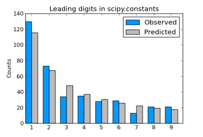
Sets of physical constants often satisfy Benford’s law, as I showed here for the constants defined in SciPy.

Incidentally, factorials satisfy Benford’s law exactly in the limit.

Weibull distributions

The Weibull distribution is a generalization of the exponential distribution. It’s a convenient distribution for survival analysis because it can have decreasing, constant, or increasing hazard, depending on whether the value of a shape parameter γ is less than, equal to, or greater than 1 respectively. The special case of constant hazard, shape γ = 1, corresponds to the exponential distribution.

Weibull and Benford

If the shape parameter of a Weibull distributions is “not too large” then samples from that distribution approximately follow Benford’s law (source). We’ll explore this statement with a little Python code.

SciPy doesn’t contain a Weibull distribution per se, but it does have support for a generalization of the Weibull known as the exponential Weibull. The latter has two shape parameters. We set the first of these to 1 to get the ordinary Weibull distribution.

      from math import log10, floor
      from scipy.stats import exponweib

      def leading_digit(x):
          y = log10(x) % 1
          return int(floor(10**y))

      def weibull_stats(gamma):

          distribution = exponweib(1, gamma)
          N = 10000
          samples = distribution.rvs(N)
          counts = [0]*10
          for s in samples:
              counts[ leading_digit(s) ] += 1

      print (counts)

Here’s how the leading digit distribution of a simulation of 10,000 samples from an exponential (Weibull with γ = 1) compares to the distribution predicted by Benford’s law.

      |---------------+----------+-----------|
      | Leading digit | Observed | Predicted |
      |---------------+----------+-----------|
      |             1 |     3286 |      3010 |
      |             2 |     1792 |      1761 |
      |             3 |     1158 |      1249 |
      |             4 |      851 |       969 |
      |             5 |      754 |       792 |
      |             6 |      624 |       669 |
      |             7 |      534 |       580 |
      |             8 |      508 |       511 |
      |             9 |      493 |       458 |
      |---------------+----------+-----------|

Looks like a fairly good fit. How could we quantify the fit so we can compare how the fit varies with the shape parameter? The most common approach is to use the chi-square goodness of fit test.

      def chisq_stat(O, E):
          return sum( (o - e)**2/e for (o, e) in zip(O, E) )

Here “O” stands for “observed” and “E” stands for “expected.” The observed counts are the counts we actually saw. The expected values are the values Benford’s law would predict:

      expected = [N*log10((i+1)/i) for i in range(1, 10)] 

Note that we don’t want to pass counts to chisq_stat but counts[1:] instead. This is because counts starts with 0 index, but leading digits can’t be 0 for positive samples.

Here are the chi square goodness of fit statistics for a few values of γ. (Smaller is better.)

      |-------+------------|
      | Shape | Chi-square |
      |-------+------------|
      |   0.1 |      1.415 |
      |   0.5 |      9.078 |
      |   1.0 |     69.776 |
      |   1.5 |    769.216 |
      |   2.0 |   1873.242 |
      |-------+------------|

This suggests that samples from a Weibull follow Benford’s law fairly well for shape γ < 1, i.e. for the case of decreasing hazard.

Related posts

Recreating the Vertigo poster

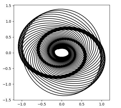
In his new book The Perfect Shape, Øyvind Hammer shows how to create a graph something like the poster for Alfred Hitchcock’s movie Vertigo.

Poster from Hitchcock's Vertigo

Hammer’s code uses a statistical language called Past that I’d never heard of. Here’s my interpretation of his code using Python.

      import matplotlib.pyplot as plt
      from numpy import arange, sin, cos, exp
      
      i  = arange(5000)
      x1 = 1.0*cos(i/10.0)*exp(-i/2500.0)
      y1 = 1.4*sin(i/10.0)*exp(-i/2500.0)
      d  = 450.0
      vx = cos(i/d)*x1 - sin(i/d)*y1
      vy = sin(i/d)*x1 + cos(i/d)*y1
      
      plt.plot(vx, vy, "k")
      
      h = max(vy) - min(vy)
      w = max(vx) - min(vx)
      plt.axes().set_aspect(w/h)
      plt.show()

This code produces what’s called a harmonograph, related to the motion of a pendulum free to move in x and y directions:

Harmonograph

It’s not exactly the same as the movie poster, but it’s definitely similar. If you find a way to modify the code to make it closer to the poster, leave a comment below.

Inverse Fibonacci numbers

As with the previous post, this post is a spinoff of a blog post by Brian Hayes. He considers the problem of determining whether a number n is a Fibonacci number and links to a paper by Gessel that gives a very simple solution: A positive integer n is a Fibonacci number if and only if either 5n2 − 4 or 5n2 + 4 is a perfect square.

If we know n is a Fibonacci number, how can we tell which one it is? That is, if n = Fm, how can we find m?

For large m, Fm is approximately φm / √ 5 and the error decreases exponentially with m. By taking logs, we can solve for m and round the result to the nearest integer.

We can illustrate this with SymPy. First, let’s get a Fibonacci number.

      >>> from sympy import *
      >>> F = fibonacci(100)
      >>> F
      354224848179261915075

Now let’s forget that we know F is a Fibonacci number and test whether it is one.

      >>> sqrt(5*F**2 - 4)
      sqrt(627376215338105766356982006981782561278121)

Apparently 5F2 – 4 is not a perfect square. Now let’s try 5F2 + 4.

      >>> sqrt(5*F**2 + 4)
      792070839848372253127

Bingo! Now that we know it’s a Fibonacci number, which one is it?

      >>> N((0.5*log(5) + log(F))/log(GoldenRatio), 10)
      100.0000000

So F must be the 100th Fibonacci number.

It looks like our approximation gave an exact result, but if we ask for more precision we see that it did not.

      >>> N((0.5*log(5) + log(F))/log(GoldenRatio), 50)
      99.999999999999999999999999999999999999999996687654

Related posts