S and C functions

I was reading a book on orbital mechanics recently [1], and one of the things that stood out was the use of two variations on sine and cosine, functions the book denotes by S and C.

\begin{align*} S(z) &= \frac{\sqrt{z} - \sin(\sqrt{z})}{\sqrt{z^3}} = \sum_{k=0}^\infty \frac{(-z)^k}{(2k+3)!} \\ C(z) &= \frac{\phantom{\sqrt{}}1 - \cos(\sqrt{z})}{z} = \sum_{k=0}^\infty \frac{(-z)^k}{(2k+2)!} \end{align*}

Strictly speaking, the functions are defined to be the analytic continuation of the middle expressions to the full complex plane, and these continuations have the given power series.

These functions come up in deriving time of flight equations. The direct derivation has expressions that would have a singularity at zero because of square root terms, and recasting the solution in terms of the functions above avoids the singularities.

(Are these functions used outside of orbital mechanics? Do they have names other than S and C? If you’ve seen them before, please let me know.)

I find these functions interesting for several reasons. First, it’s interesting that the power series for the two functions are so similar.

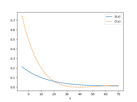
Second, the functions S and C are derived from sine and cosine, but you might not guess that from looking at their plots.

The power series forms of the two functions are similar, but the plots of the two functions are not.

Third, you might expect the derivative of a sine-like thing to be a cosine-like thing and vice versa. Well, that’s sorta true in our case. The derivatives of S and C are related to the functions S and C, but its a little complicated.

\begin{align*} S'(z) &= \frac{1}{2z} (C - 3S) \\ C'(z) &= \frac{1}{2z} (1 - 2C - zS) \end{align*}

Maybe it’s surprising that the relationship is as complicated as it is, or maybe it’s surprising that it’s not more complicated.

Finally, when z is a real variable, we can evaluate S with

S(x) = \left\{ \begin{array}{ll} \big(\sqrt{x} - \sin(\sqrt{x})\big)/\sqrt{x^3} & \mbox{if } x > 0 \\ 1/6 & \mbox{if } x = 0 \\ \big(\sinh(\sqrt{-x})- \sqrt{-x}\big)/\sqrt{(-x)^3} & \mbox{if } x < 0 \end{array} \right.

and evaluate C with

C(x) = \left\{ \begin{array}{ll} \big(1-\cos\sqrt{x}\big)/x & \mbox{if } x > 0 \\ 1/2 & \mbox{if } x = 0 \\ \big(1-\cosh\sqrt{-x}\big)/x & \mbox{if } x < 0 \end{array} \right.

Written this way, it looks like the functions S and C are arbitrarily patched together. But the functions are smooth at 0, even analytic at 0 as the power series shows. The equations are not arbitrary at all but uniquely determined.

Update: Someone contributed this post to Hacker News and someone else left a helpful comment with some historical background. Apparently this work goes back to Karl Stumpff and was written up in a NASA technical report. It was further developed at MIT and written up in a textbook by Richard Battin.

More orbital mechanics posts

[1] Fundamentals of Astrodynamics by Roger R Bate, Donald D. Mueller, and Jerry E. White. Dover, 1971.

Offline documentation

It’s simpler to search the web than to search software-specific documentation. You can just type your query into a search engine and not have to be bothered by the differences in offline documentation systems for different software. But there are a couple disadvantages.

First, the result may not be that relevant. For example, maybe you have a question about LaTeX typesetting and you get back results about rubber. And even if the result is relevant, it might not be accurate or up-to-date.

Second, you might not always be online. You might lose your internet connection, or you might deliberately stay offline for a block of time in order to concentrate better.

A convenient way to grab online documentation for a lot of software packages is to use Dash for macOS or Zeal on Windows and Linux.

If you use a particular piece of software a lot, you probably want to learn how to use its native documentation system. It’s hard to do this for lots of different tools, hence the popularity of the generic web search, but it’s worthwhile for a small number of high priority tools.

Engineering attitude

Carver Mead on engineering:

Engineering isn’t something you study and learny, and memorize, and know where to look up. Engineering is understanding things all the way to the bottom, no matter what field they are called, and being able use that to build stuff and make it work.

I edited the quote slightly. Mead was speaking in the past tense about the attitude that Royal Sorensen brought to Cal Tech. I thought the stand-alone quote would be easier to read in the present tense.

Source: Carver Mead: the thing that’s going to be the most important 100 years from now, around 22:30.

Searching for pseudoprimes

I was reading a book on computer algebra and ran across an interesting theorem about Carmichael numbers in the one of the exercises. I’ll present that theorem below, but first I’ll back up and say what a pseudoprime is and what a Carmichael number is.

Fermat’s theorem

If p is a prime number, then for any integer b, Fermat’s little theorem says

bp-1 = 1 (mod p).

The contrapositive of this theorem is useful for testing whether a number is (not) prime: if for some b,

bp-1 ≠ 1 (mod p)

then p is not a prime. For example, we could test whether 1003 is prime by computing [1]

21002 (mod 1003).

When we do, we find the result is 990, not 1, and so 1003 is not prime.

Pseudoprimes

Let’s test whether 341 is prime. If we compute

2340 (mod 341)

we get 1. But clearly 341 = 11 × 31. If we go back and read the top of the post carefully, we see that Fermat’s theorem only gives a way to prove a number is not prime. We say 341 is a pseudoprime base 2 because it is a composite number that slips past the primality test based on Fermat’s little theorem with b = 2.

Strictly speaking we should say 341 is a Fermat pseudoprime base 2. When someone says “pseudoprime” without further qualification, they usually mean Fermat pseudo prime. But there are other kinds of pseudoprimes. For any theorem that gives a necessary but not sufficient for a number to be prime, the composite numbers that satisfy the condition are called pseudoprimes. See this post for examples, such as Euler pseudoprimes and Wilson pseudoprimes.

Note that 341 is not a Fermat pseudoprime base 3 because

3340 = 56 (mod 341)

If a number passes Fermat’s primality test for several bases, it’s probably prime. (Here’s a blog post that carefully unpacks what “probably prime” means.)

Carmichael numbers

We saw that 341 is a Fermat pseudoprime for base 2 but not base 3; it slipped past our first check on primality but not our second. Some numbers are more slippery. Carmichael numbers are composite numbers that slip past Fermat’s primality test for every base b.

Actually, not every base. A Carmichael number n passes Fermat’s primality test for any base b relatively prime to n.

The smallest Carmichael number is 561. There are infinitely many Carmichael numbers, but they’re distributed very thinly.

Searching for Carmichael numbers

Now I’m finally ready to get to the exercise I mentioned at the top of the post. I’m reading Computer Algebra by Wolfram Koepf. The exercise asks the reader to prove that if for a given k the three numbers 6k+1, 12k+1, and 18k+1 are all prime, then their product is a Carmichael number. This theorem was discovered by J. Chernick in 1939.

We can use this to search for Carmichael numbers with the following Python code. (Note that this approach doesn’t produce all Carmichael numbers—it doesn’t produce 561, for example.) It is unknown whether it produces an infinite sequence of Carmichael numbers.

    from sympy import isprime

    for k in range(2, 100):
        if isprime(6*k+1) and isprime(12*k+1) and isprime(18*k+1):
            print(k, (6*k+1)*(12*k+1)*(18*k+1))

Testing values of k up to 100 reveals six Carmichael numbers.

     6 294409
    35 56052361
    45 118901521
    51 172947529
    55 216821881
    56 228842209

Related posts

[1] This may not look like a good idea at first. 21002 is an enormous number. Surely it would be easier to test whether 1003 is prime than to compute such a large number. Except you don’t have to compute 21002 per se: you have to compute 21002 (mod 1003). You can reduce your intermediate results (mod 1003) at every step, so you never have to work with large numbers. You can also use fast exponentiation, and so Fermat’s primality test is much more efficient than it may seem at first glance.

Python’s pow function optionally takes a modulus as a third argument. So, for example,

    pow(2, 1002)

computes 21002, and

    pow(2, 1002, 1003)

computes 21002 (mod 1003). It produces the same result as

    2**1002 % 1003

but is more efficient. Not that it matters in this example, but it matters more when the exponent is much larger.

Finding computer algebra algorithms with computer algebra

I ran across an interesting footnote in Wolfram Koepf’s book Computer Algebra.

Gosper’s algorithm [1] was probably the first algorithm which would not have been found without computer algebra. Gosper writes in his paper: “Without the support of MACSYMA and its developer, I could not have collected the experiences necessary to provoke the conjectures that lead to the algorithm.”

When I first glanced at the footnote I misread it, coming away with the impression that Gosper said he could not have proved that his algorithm was correct without computer algebra. But he said he would not have formulated his algorithm without his experience using MACSYMA.

If a sum of hypergeometric terms is itself hypergeometric, Gosper’s algorithm gives a way to find the sum. Gosper’s algorithm, discovered using computer algebra, is itself an important computer algebra algorithm.

Related posts

[1] Koepf cites Gosper as R. W. Gosper, Jr. Decision procedure for indefinite hypergeometric summation. Proc. Natl. Acad. Sci. USA, 75, 1978, 40–42.

Approximate minimal bounding sphere

Problem statement

Suppose you have a large number of points in 3D space and you want to find a sphere containing all the points. You’d like the sphere to be as small as possible, but you’re willing to accept a slightly larger sphere in exchange for simplicity or efficiency.

False starts

If you knew the center of the sphere, the solution would be easy: find the distance from every point to the center, and the large distance is the radius. But you don’t know the center of the bounding sphere when you start.

What if you found the two points the furthest apart from each other? Maybe that would give you the diameter of the bounding sphere, and the center would be the midpoint of the line connecting these two points.

There are a couple problems with this approach. First, how would you find the two points furthest from each other? The most obvious approach would be to compute the distance between all pairs of points. But if you have n points, you have n(n+1)/2 pairs of points. That would make the algorithm O(n²).

If you do know the two points that are furthest apart, that gives you a lower bound on the diameter of the bounding sphere, but not the diameter itself. For example, suppose we’re working in two dimensions and discover that the longest line between two points connects (-10, 0) and (10, 0). You might try centering a circle of radius 10 at the origin. But what if there’s a third point (0, 11)? It doesn’t change which two points are maximally distance, but it’s a distance of 11 from the origin.

Jack Ritter’s algorithm

A fairly simple algorithm by Jack Ritter runs in linear time, i.e. O(n), and is guaranteed to produce a sphere containing the given points. But the sphere it returns might be a little bigger than necessary. Ritter says [1] “the sphere calculated is about 5% bigger than the ideal minimum-radius sphere.”

When I read that, my first thought was “What kind of distribution is he assuming on points to come up with that 5% estimate?” The expected efficiency of the algorithm must depend on the the distribution on the input points.

Ritter gives two examples. The first started with a sphere “randomly populated with 100,000 points.” Random according to what distribution? I assume uniform. The calculated sphere had a radius 4% larger than optimal. The second example was a cube “randomly populated with 10,000 points.” Again I assume the distribution was uniform. The calculated sphere had a radius that was 7% larger than optimal.

I’ve seen a couple sources that say Ritter’s algorithm is between 5% and 20% from optimal. I’m curious what the 20% figure is based on; the examples below fit much better than that. Maybe the fit is worse for point sets with less symmetry. The number of points may also effect the expected efficiency.

Testing Ritter’s algorithm

To test Ritter’s algorithm, I grabbed an implementation in Python from here. (There’s a flaw in this implementation. See update below.)

Cube example

First, I took 10,000 uniform samples from the unit cube. I started with this example since sampling from a cube is easy.

I changed the last four of the random samples to be corners of the cube so I’d know the exact answer.

    from scipy.stats import uniform
    x = uniform.rvs(size=(10000, 3)).tolist()
    x[-1] = [0, 0, 0]
    x[-2] = [0, 0, 1]
    x[-3] = [1, 0, 0]
    x[-4] = [1, 1, 1]
    print( bounding_sphere(x) )

This returned a sphere of radius 0.8772 centered at (0.5010, 0.4830, 0.4968). The exact solution is a sphere of radius 0.5√3 centered at (0.5, 0.5, 0.5). The radius of the computed sphere was only 1.3% greater than optimal. I repeated my experiment 10 times and the worst fit was 2.2% greater than optimal. It seems Ritter’s cube experiment result was either unlucky or flawed, and in either case pessimistic.

Sphere example

Next I wanted to generate around 10,000 points uniformly from a sphere of radius 0.5 centered at (0.5, 0.5, 0.5). I did this by generating points from the unit cube and throwing away those that weren’t in the sphere I was after [2]. The sphere takes up about half of the unit cube, so I generated 20,000 points in order to have about 10,000 that landed inside the sphere.

    def inside(c):
        return (c[0]-0.5)**2 + (c[1]-0.5)**2 + (c[2]-0.5)**2 < 1/4

    cube = uniform.rvs(size=(20000, 3)).tolist()
    x = [c for c in cube if inside(c)]
    x[-1] = [0.5, 0.5, 0.0]
    x[-2] = [0.0, 0.5, 0.5]
    x[-3] = [0.5, 0.0, 0.5]
    x[-4] = [0.5, 1.0, 0.5]
    print( bounding_sphere(x) )

This returned a sphere of radius 0.5282 centered at (0.4915, 0.4717, 0.4955). This radius is about 5.6% larger than the optimal radius of 0.5.

I repeated the experiment 10 times, and on average the spheres were 5% larger than optimal. The worst case was 7.6% larger than optimal.

Update

Thanks to Chris Elion for pointing out that the implementation of Ritter’s algorithm that I found does not fully implement the algorithm: it does not update the center as Ritter does in [1].

Chris reran the calculations above and in each case roughly cut the distance between the computed and optimal radius in half.

Related posts

[1] Graphics Gems. Andrew S. Glassner, editor. Academic Press. 1990.

[2] There’s an apocryphal quote attributed to Michelangelo that when asked how he carved David, he said that he started with a block of marble and cut away everything that wasn’t David. In probability this approach is known as acceptance-rejection sampling. It’s simple, but not always the most efficient approach.
Complex floor and a surprising pattern

The floor of a real number x, written ⌊x⌋, is the largest integer less than or equal to x. So, for example, ⌊π⌋ = 3 and ⌊-π⌋ = -4.

The previous post applied the floor function to a complex number z. What does that mean? You can’t just say it’s the largest integer [1] less than z because the complex numbers aren’t ordered; there’s no natural way to say whether one complex number is less than or greater than another.

The post was using Mathematica code, and Mathematica defines the floor of a complex number by applying the function to the real and imaginary parts separately. That is, if x and y are real numbers, then

x + iy⌋ = ⌊x⌋ + iy⌋.

That lets you take the floor of a complex number, but is it useful? I wondered how many identities that hold for floors of real numbers extend to complex numbers when the floor is defined as above, so I looked at the chapter in Concrete Mathematics that has a bunch of identities involving floors and ceilings to see which ones extend to complex numbers.

Any identity where the real an imaginary parts don’t interact should extend trivially. For example, for real x and integer n,

x + n⌋ = ⌊x⌋ + n.

This extends to the case where x is complex and n is a (complex) integer [1]. Addition works on real and imaginary components separately, just like Mathematica’s definition of floor.

But here’s one that’s much more interesting. For positive x,

⌊√⌊x⌋ ⌋ = ⌊√x⌋.

Taking square roots deeply intertwines the real and imaginary parts of a number [3]. Does the identity above hold for complex inputs?

I wrote some Python code to test this, and to my great surprise, the identity often holds. In my first experiment, it held something like 84% of the time for random inputs. I expected it would either rarely hold, or hold say half the time (e.g. in a half-plane).

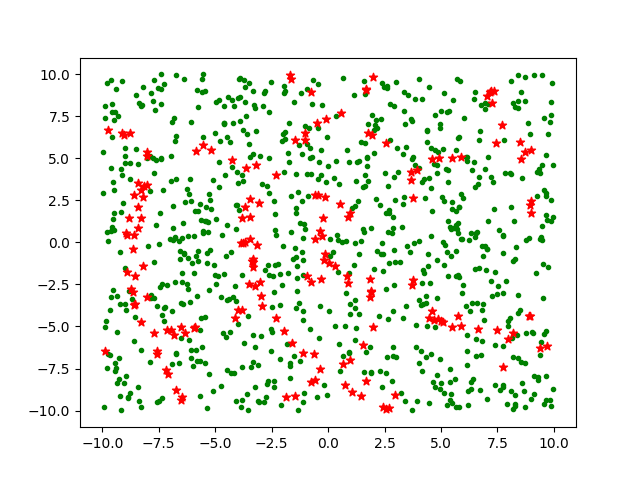
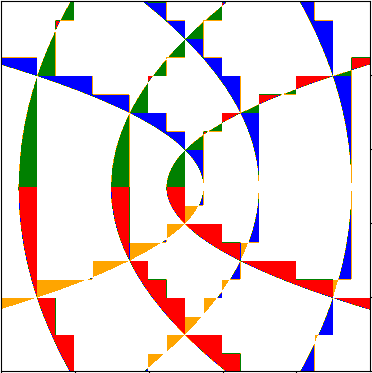
My first thought was to plot 1,000 random points, green dots where the identity holds and red stars where it does not. This produced the following image.

Red stars scattered randomly among green dots

About 16% of the points are red and the rest green. In this plot there’s no apparent pattern to the red points.

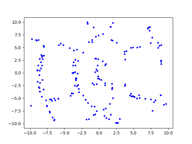
Since I’m sampling uniformly throughout the square, there’s no reason to plot both where the identity holds and where it doesn’t. So for my next plot I just plotted where the identity fails.

Red stars scattered randomly among green dots

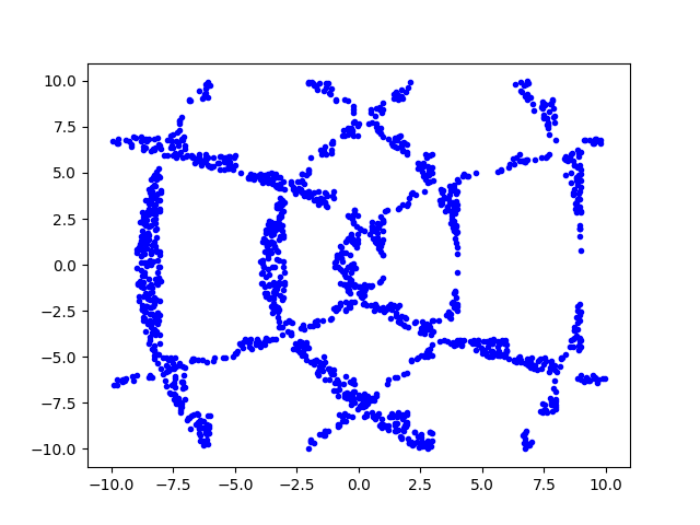
That’s a little  clearer. To make it clearer, I rerun the plot with 10,000 samples. (That’s the total number of random samples tested, about 16% of which are plotted.)

Red stars scattered randomly among green dots

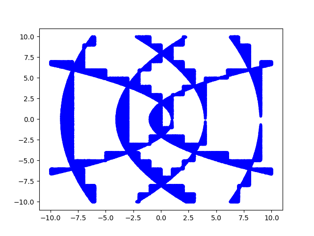
Then to improve the resolution even more, I increased the number of samples to 1,000,000.

Red stars scattered randomly among green dots

It might not be too hard to work out analytically the regions where the identity holds and doesn’t hold. The blue regions above look sorta like parabolas, which makes sense because square roots are involved. And these parabola-like curves has ziggurat-like embellishments, which makes sense because floors are involved.

Update

Define

f(z) = ⌊√⌊z⌋ ⌋ – ⌊√z⌋.

The graphs above plotted the set of zs for which f(z) ≠ 0. We can see more information by plotting f itself. The function only takes on five possible values: 0, 1, i, -1, and –i. I plotted these as white, orange, green, blue, and red.

Related posts

[1] You could extend the meaning of “integer” to a complex number with integer real and imaginary parts, commonly known as a Gaussian integer.

[2] I suspect Mathematica’s definition is not common. I don’t know of any other source that even defines the floor of a complex number, much less defines it as Mathematica does.

[3] You may be wondering what’s going on with the square root. Complex numbers have two square roots, so which one(s) are we using? I’m doing what Python does, taking the principal branch. That is, using the analytic continuation of square root that extends from the real axis to the complex plane with the negative real axis excluded.

Plotting the Gauss map

A recent post looked at an example from one of Michael Trott’s tomes. This post looks at another example from the same tome.

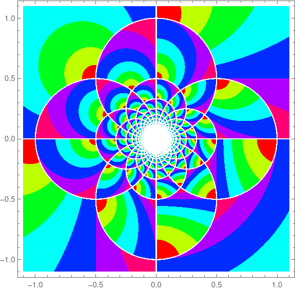
Trott made a contour plot of the Gauss map

f(x) = \frac{1}{x} - \left\lfloor \frac{1}{x}\right\rfloor

over the complex plane. I copied his code (almost) and reproduced his plot.

    ContourPlot[
        Abs[1/(x + I y) - Floor[1/(x + I y)]], 
        {x, -1.1, 1.1}, {y, -1.1, 1.1}, 
        PlotPoints -> 40, ColorFunction -> Hue, 
        ContourStyle -> {Thickness[0.00001]}
    ]

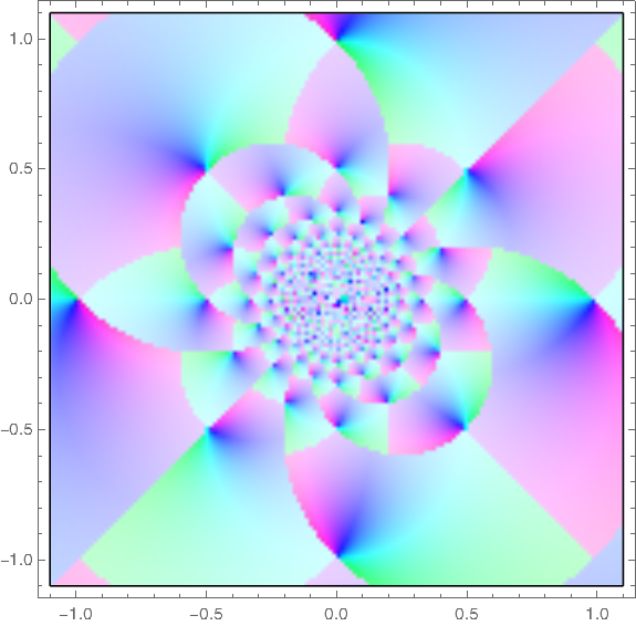
This produced the following image.

The original code set PlotPoints to 400, and it was taking forever. I got impatient and set the parameter to 40. Looking at the image in the book, it seems the plot with the parameter set to 400 is very similar, except there’s a black tangle in the middle rather than a white space.

In 2004 when Trott wrote his book, Mathematica did not have a command for plotting functions of a complex variable directly, and so Trott rolled his own as a function of two real variables.

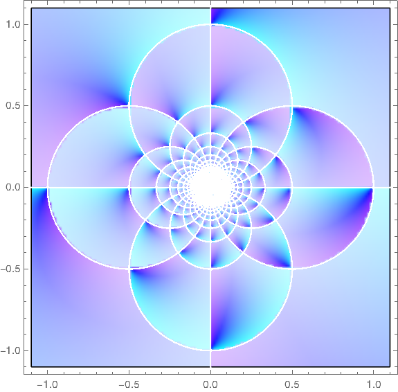
Here’s a plot of the same function using the relatively new ComplexPlot function.

Here’s the code that produced the plot.

    ComplexPlot[
        (1/z - Floor[1/z]), 
        {z, -1.1 - 1.1 I, 1.1 + 1.1 I}, 
        ColorFunction -> Hue, PlotPoints -> 400
    ]

Update

What does it mean to apply the floor function to a complex number? See the next post.

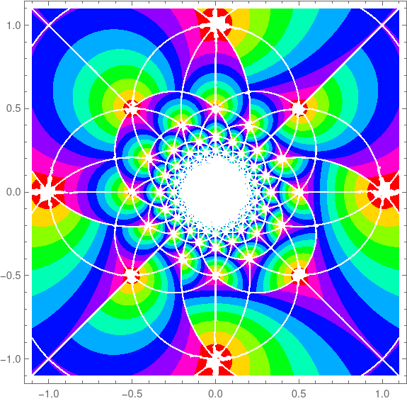
The plots above were based on Mathematica’s definition of complex floor. Another definition gives different plots.

    aplfloor[z_] := 
        With[ {x = Re[z] - Floor[Re[z]], y = Im[z] - Floor[Im[z]], g = Floor[z]}, 
        If[x + y > 1, If[x >= y, g + 1, g + I], g]]

This leads to different plots of the Gauss map.

Vintage:

And new style:

Related posts

Collatz analog in C

A few days ago I wrote about an analog of the Collatz conjecture for polynomials with coefficients mod m. When m = 2, the conjecture is true, but when m = 3 the conjecture is false.

I wrote some Mathematica code on that post to work with polynomials as polynomials. Then a comment on that post made me realize that the m = 2 case could easily be implemented in integers using bit shifts and XOR.

Recall that the rule was that if p(x) has a constant term, multiply by (x + 1) and add 1. Otherwise divide by x.

It’s easy to represent polynomials mod 2 as integers: set the nth bit from the right to 1 if and only if the coefficient of xn is 1. This assumes we’re counting from 0. Dividing by x corresponds to shift bits to the right, and multiplying by x corresponds to shifting bits to the left. Polynomial addition corresponds to XOR.

So here’s the Collatz operation in verbose C:

    if (x != 1)
        if (x & 1)
            x = x ^ (x << 1) ^ 1;
        else
            x >>= 1;

Here it is in terse C:

    (x == 1) ? 1 : (x & 1) ? x ^ (x << 1) ^ 1 : x >> 1;

Due to the operator precedent rules for C, all the parentheses can be removed, resulting in even more terse/cryptic code.

    x == 1 ? 1 : x & 1 ? x ^ x << 1 ^ 1 : x >> 1;

The left shift above can overflow, and it’s not clear how large the inputs to this iteration can be. We know that the iterates will eventually converge to 1, but it’s not obvious how large the iterations can get before they start getting smaller.

3D bifurcation diagram

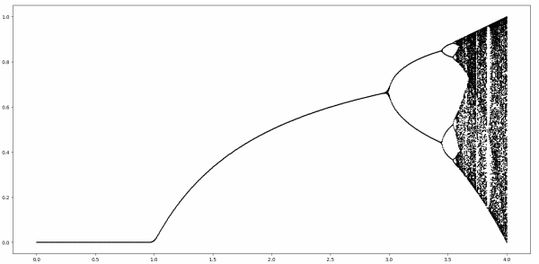
The following 2D bifurcation diagram is famous. You’ve probably seen it elsewhere.

logistic bifurcation diagram

If you have seen it, you probably know that it has something to do with chaos, iterated functions, fractals, and all that. If you’d like to read in more detail about what exactly the plot means, see this post.

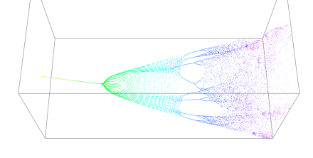
I was reading Michael Trott’s Mathematica Guidebook for Numerics and ran across a 3D version of the above diagram. I’d never seen that before. He plots the iterations of the system

x ← a – y(β x + (1 – β) y)
yx + y²/100

The following plot is for β = 1/4 using the code included in the book. (I changed the parameter α in the book to β because the visual similarity between a and α was a little confusing.)

Trott cites four papers regarding this iteration. I looked at a couple of the papers, and they contain similar systems but aren’t quite the same. Maybe his example is a sort of synthesis of the examples he found in the literature.

Related posts: More on dynamical systems