Bluesky

I saw a comment from Christos Argyropoulos on Twitter implying that there’s a good scientific community on Bluesky, so I went there and looked around a little bit. I have account, but I haven’t done much with it. I was surprised that a fair number of people had followed me on Bluesky even though I only posted twice. I posted a couple links this evening, doubling my total activity on Bluesky.

I don’t know what I’ll do with my Bluesky or Mastodon accounts. I certainly will not try to replicate what I built on Twitter. So far I’m more of a reader than a writer on Bluesky and Mastodon. Bluesky is not a science-focused social network, but I may use it for that, only following science-oriented accounts there. We’ll see.

You can always find me here, whether or not you can find me on Bluesky, Mastodon, or Twitter. You can subscribe to this site to get notifications of new posts via RSS or email, and I also have a monthly newsletter where I post blog highlights.

Portable sed -i across MacOS and Linux

The -i flag to ask sed to edit a file in place works differently on Linux and MacOS. If you want to create a backup of your file before you edit it, say with the extension .bak, then on Linux you would run

    sed -i.bak myfile

but for the version of sed that ships with MacOS you would write

    sed -i '.bak' myfile

Note that this changes how sed interprets its arguments, whether you want a backup file or not. You must specify a backup file extension, but could specify the extension as '', which effectively means don’t make a backup.

The difference between how the two versions of sed handle their arguments is a minor nuisance when working interactively at the command line, but a script calling sed -i will not work the same on Mac and Linux.

I put the line

   alias sed=gsed

in my .zshrc file so that when I type sed the shell will actually run the Gnu version of sed, which handles -i as I expect.

But this does not work in bash scripts. I tried putting the alias in my .bashrc and .bash_profile files, but that doesn’t work. In scripts bash ignores aliases, no matter what config file you put them in. Here’s the relevant line from the bash man page:

Aliases are not expanded when the shell is not interactive, unless the expand_aliases shell option is set using shopt.

So the solution is to put the magic incantation

   shopt -s expand_aliases

at the top of your script.

Here’s how I wrote a script using sed -i works the same way on MacOS and Linux.

    #!/usr/bin/env bash
    shopt -s expand_aliases

    if [[ "$OSTYPE" == "darwin"* ]]; then
        alias sed=gsed
    fi

    sed -i ...

This may seem a little heavy-handed, changing the program that I’m using just to fix a problem with the arguments. I could, for example, have the script insert '' after -i when running on MacOS.

But I’m not changing the program I use. Quite the opposite. The code above saves me from having to use a different program. It insures that I’m running the Gnu version of sed on both platforms. There are other differences between the two versions of sed. I don’t know what they are off hand, but they could lead to frustrating bugs in the future, and the code above fixes these bugs before they occur.

Johnson circle theorem

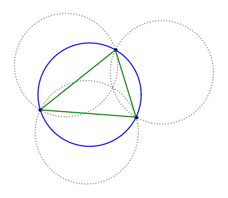
Draw three circles of radius r that intersect at a single point. Then draw a triangle connecting the remaining three points of intersection.

(Each pair of circles intersects in two points, one of which is the point where all three circles intersect, so there are three other intersection points.)

Then the circumcircle of the triangle, the circle through the three vertices, also has radius r.

I’ve seen this theorem referred to as Johnson’s theorem, as well as the Johnson–Tzitzeica or Tzitzeica-Johnson theorem. Apparently Roger Johnson and George Tzitzeica (Gheorghe Țițeica) both proved the same theorem around the same time. Johnson’s publication [1] dates to 1916.

It’s remarkable that a theorem in Euclidean geometry this easy to state was discovered 2200 years after Euclid. Johnson says in [1]

Singularly enough, this remarkable theorem appears to be new. A rather cursory search in several of the treatises on modern elementary geometry fails to disclose it, and the author has not yet found any person to whom it was known. On the other hand, the figure is so simple … that it seems almost out of the question that the fact can have escaped detection. Even if geometers have overlooked it, someone must have noticed it in casually drawing circles. But if this were the case, it seems like a theorem of sufficient interest to receive some prominence in the literature, and therefore ought to be well known.

Related posts

[1] Roger Johnson. A circle theorem. The American Mathematical Monthly, May, 1916, Vol. 23, No. 5, pp. 161-162.

Newton line

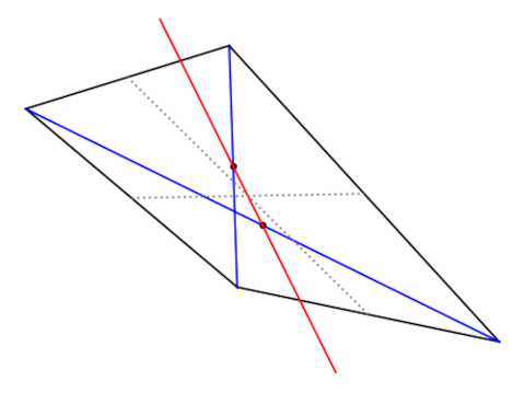
Let Q be a convex quadrilateral with at most two parallel sides. Draw the two diagonals then draw a line through their midpoints. This line is called the Newton line.

(The requirement that at most two sides are parallel insures that the midpoints are distinct and so there is a unique line joining them.)

In the figure above, the diagonals are blue, their midpoints are indicated by black dots, and the red line joining them is the Newton line.

Now join the midpoints of the sides. These are draw with dotted gray lines above. Then the intersection of these two lines lies on the Newton line.

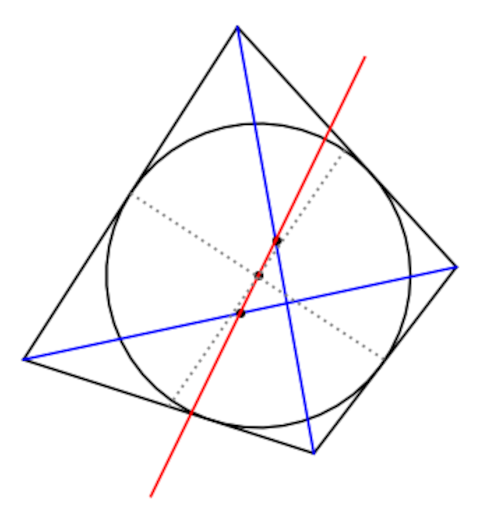
Now suppose further that our quadrilateral is a tangential quadrilateral, i.e. that all four sides are tangent to a circle C. Then the center of C also lies on the Newton line.

In the image above, it appears that the lines joining the midpoints of the sides also passes intersect at the center of the circle. That’s not true in general, and its not true in the example above but you’d have to zoom in to see it. But it is true that the intersection of these lines and the center of the circle both lie on the Newton line.

Related posts

Homework problems are rigged

This post is a follow-on to a discussion that started on Twitter yesterday. This tweet must have resonated with a lot of people because it’s had over 250,000 views so far.

You almost have to study advanced math to solve basic math problems. Sometimes a high school student can solve a real world problem that only requires high school math, but usually not.

There are many reasons for this. For one thing, formulating problems is a higher-level skill than solving them. Homework problems have been formulated for you. They have also been rigged to avoid complications. This is true at all levels, from elementary school to graduate school.

A college school student tutoring a high school student might notice that homework problems have been crafted to always have whole number solutions. The college student might not realize how his own homework problems have been rigged analogously. Calculus homework problems won’t avoid fractions, but they still avoid problems that don’t have tidy solutions [1].

When I taught calculus, I looked around for homework problems that were realistic applications, had closed-form solutions, and could be worked in a reasonable amount of time. There aren’t many. And the few problems that approximately satisfy these three criteria will be duplicated across many textbooks. I remember, for example, finding a problem involving calculating the mass of a star that I thought was good exercise. Then as I looked through a stack of calculus texts I saw that the same homework problem was in most if not all the textbooks.

But it doesn’t stop there. In graduate school, homework problems are still crafted to avoid difficulties. When you see a problem like this one it’s not obvious that the problem has been rigged because the solution is complicated. It may seem that you’re able to solve the problem because of the power of the techniques used, but that’s not the whole story. Tweak any of the coefficients and things may go from complicated to impossible.

It takes advanced math to solve basic math problems that haven’t been rigged, or to know how to do your own rigging. By doing your own rigging, I mean looking for justifiable ways to change the problem you need to solve, i.e. to make good approximations.

For example, a freshman physics class will derive the equation of a pendulum as

y″ + sin(y) = 0

but then approximate sin(y) as y, changing the equation to

y″ + y = 0.

That makes things much easier, but is it justifiable? Why is that OK? When is that OK, because it’s not always.

The approximations made in a freshman physics class cannot be critiqued using freshman physics. Working with the un-rigged problem, i.e. keeping the sin(y) term, and understanding when you don’t have to, are both beyond the scope of a freshman course.

Why can we ignore friction in problem 5 but not in problem 12? Why can we ignore the mass of the pulley in problem 14 but not in problem 21? These are questions that come up in a freshman class, but they’re not freshman-level questions.

***

[1] This can be misleading. Students often say “My answer is complicated; I must have made a mistake.” This is a false statement about mathematics, but it’s a true statement about pedagogy. Problems that haven’t been rigged to have simple solutions often have complicated solutions. But since homework problems are usually rigged, it is true that a complicated result is reason to suspect an error.

Python code for means

The last couple article have looked at various kinds of mean. The Python code for four of these means is trivial:

gm  = lambda a, b: (a*b)**0.5
am  = lambda a, b: (a + b)/2
hm  = lambda a, b: 2*a*b/(a+b)
chm = lambda a, b: (a**2 + b**2)/(a + b)

But the arithmetic-geometric mean (AGM) is not trivial:

from numpy import pi
from scipy.special import ellipk

agm = lambda a, b: 0.25*pi*(a + b)/ellipk((a - b)**2/(a + b)**2) 

The arithmetic-geometric mean is defined by iterating the arithmetic and geometric means and taking the limit. This iteration converges very quickly, and so writing code that directly implements the definition is efficient.

But the AGM can also be computed via a special function K, the “complete elliptic integral of the first kind,” which makes the code above more compact. This is conceptually nice because we can think of the AGM as a simple function, not an iterative process.

But how is K evaluated? In some sense it doesn’t matter: it’s encapsulated in the SciPy library. But someone has to write SciPy. I haven’t looked at the SciPy source code, but usually K is calculated numerically using the AGM because, as we said above, the AGM converges very quickly.

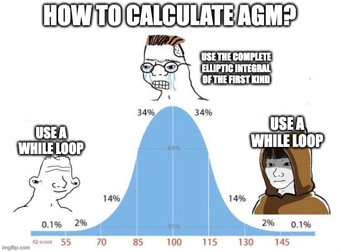
Bell curve meme: How to calculate the AGM? The left and right tails say to use a while loop. The middle says to evaluate a complete ellliptic integral of the first kind.

This fits the pattern of a bell curve meme: the novice and expert approaches are the same, but for different reasons. The novice uses an iterative approach because that directly implements the definition. The expert knows about the elliptic integral, but also knows that the iterative approach suggested by the definition is remarkably efficient and eliminates the need to import a library.

Although it’s easy to implement the AGM with a while loop, the code above does have some advantages. For one thing, it pushes the responsibility for validation and exception handling onto the library. On the other hand, the code is easy to get wrong because there are two conventions on how to parameterize K and you have to be sure to use the same one your library uses.

More ways of splitting the octave

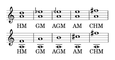
in an earlier post I said that the arithmetic mean of two frequencies an octave apart is an interval of a perfect fifth, and the geometric mean gives a tritone. This post will look at a few other means.

Intervals

The harmonic mean (HM) gives a perfect fourth.

The arithmetic-geometric mean (AGM) gives a pitch about midway between a tritone and a fifth, a tritone plus 50 cents.

The arithmetic mean gives a perfect fifth.

The contraharmonic mean gives an interval of a major sixth.

The intervals for HM, AM, and CHM are exact, using just tuning. The intervals for GM is exact using equal temperament. The AGM is not close to a chromatic tone in any system.

If we take the means of A 440 and A 880, the AGM is an E half-flat (hence the backward flat sign above).

Equations

Here are the equations for the various means:

\begin{align*} HM(a, b) &= \frac{2ab}{a + b} \\ GM(a, b) &= \sqrt{ab} \\ AM(a, b) &= (a + b)/2 \\ CHM(a, b) &= \frac{a^2 + b^2}{a + b} \end{align*}

The AGM is defined iteratively: Take the GM and AM of the pair of numbers, then take the GM and AM of the result, and so on, taking the limit. More detail here.

Frequencies

Here are the frequencies of the means.

    |------+-----|
    | Mean |  Hz |
    |------+-----| 
    | HM   | 586 |
    | GM   | 622 |
    | AGM  | 641 |
    | AM   | 660 |
    | CHM  | 733 |
    |------+-----|

Lilypond

Here’s the Lilypond code that was used to create the music notaton above.

\begin{lilypond}

\new Staff \with { \omit TimeSignature} {
  \relative c''{
     <a d>1 <a ees'>1 <a eeh'>1 <a e'>1 <a fis'>1 |
  }
  \addlyrics{"HM" "GM" "AGM" "AM" "CHM" }
}

\end{lilypond}

Update: Two octaves

What if we look at frequencies two octaves apart, 220 Hz and 880 Hz? You might expect the size of the intervals to double. That intuition is exactly correct for the geometric mean: a tritone is half an octave (on a log scale) and so two tritones is an octave.

This intuition is also approximately correct for the arithmetic-geometric mean. But it over-estimates the harmonic mean and under-estimates the arithmetic and contraharmonic means.

Maclaurin’s inequality

This afternoon I wrote a brief post about Terence Tao’s new paper A Maclaurin type inequality. That paper builds on two classical inequalities: Newton’s inequality and Maclaurin’s inequality. The previous post expanded a bit on Newton’s inequality. This post will do the same for Maclaurin’s inequality.

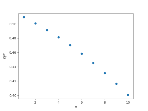
As before, let x be a list of real numbers and define Sn(x) to be the average over all products of n elements from x. Maclaurin’s inequality says that Sn(x)1/n is decreasing function of n.

S1(x) ≥ S2(x)1/2S3(x)1/3 ≥ …

We can illustrate this using the Python code used in the previous post with a couple minor changes. We change the definition of ys to

   ys = [S(xs, n)**(1/n) for n in ns]

and change the label on the vertical axis accordingly.

Looks like a decreasing function to me.

Newton’s inequality and log concave sequences

The previous post mentioned Newton’s inequality. This post will explore this inequality.

Let x be a list of real numbers and define Sn(x) to be the average over all products of n elements from x. Newton’s inequality says that

Sn−1 Sn+1S²n

In more terminology more recent than Newton, we say that the sequence Sn is log-concave.

The name comes from the fact that if the elements of x are positive, and hence the S‘s are positive, we can take the logarithm of both sides of the inequality and have

(log Sn−1 + log Sn+1)/2 ≤ log Sn

which is the discrete analog of saying log Sk is concave as a function of k.

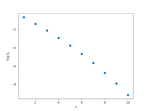
Let’s illustrate this with some Python code.

from itertools import combinations as C
from numpy import random
from math import comb
import matplotlib.pyplot as plt

def S(x, n):
    p = lambda c: prod([t for t in c])
    return sum(p(c) for c in C(x, n))/comb(N, n)

random.seed(20231010)
N = 10
xs = random.random(N)
ns = range(1, N+1)
ys = [log(S(xs, n)) for n in ns]

plt.plot(ns, ys, 'o')
plt.xlabel(r"$n$")
plt.ylabel(r"$\log S_n$")
plt.show()

This produces the following plot.

This plot looks nearly linear. It’s plausible that it’s concave.