First names and Bayes’ theorem

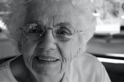
Is the woman in this photograph more likely to be named Esther or Caitlin?

black and white photo of an elderly woman

Yesterday Mark Jason Dominus published wrote about statistics on first names in the US from 1960 to 2021. For each year and state, the data tell how many boys and girls were given each name.

Reading the data “forward” you could ask, for example, how common was it for girls born in 1960 to be named Paula. Reading the data “backward” you could ask how likely it is that a woman named Paula was born in 1960.

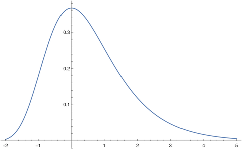
We do this intuitively. When you hear a name like Blanche you may think of an elderly woman because the name is uncommon now (in the US) but was more common in the past. Sometimes we get a bimodal distribution. Olivia, for example, has made a comeback. If you hear that a female is named Olivia, she’s probably not middle aged. She’s more likely to be in school or retired than to be a soccer mom.

Bayes’ theorem tells us how to turn probabilities around. We could go through Mark’s data and compute the probabilities in reverse. We could quantify the probability that a woman named Paula was born in the 1960s, for example, by adding up the probabilities that she was born in 1960, 1961, …, 1969.

Bayes theorem says

P(age | name) = P(name | age) P(age) / P(name).

Here the vertical bar separates the thing we want the probability of from the thing we assume. P(age | name), for example, is the probability of a particular age, given a particular name.

There is no bar in the probability in the denominator above. P(name) is the overall probability of a particular name, regardless of age.

People very often get probabilities backward; they need Bayes theorem to turn them around. A particular case of this is the prosecutor’s fallacy. In a court of law, the probability of a bit of evidence given that someone is guilty is irrelevant. What matters is the probability that they are guilty given the evidence.

In a paternity case, we don’t need to know the probability of someone having a particular genetic marker given that a certain man is or is not their father. We want to know the probability that a certain man is the father, given that someone has a particular genetic marker. The former probability is not what we’re after, but it is useful information to stick into Bayes’ theorem.

Related posts

Photo by Todd Cravens on Unsplash.

Identifiable to man or machine?

Like the previous post, this post riffs on a photo [1] I stumbled on while looking for something else.

Would it be easier to identify the man in this photo or the man whose photo appeared in the previous post, copied below.

I think it would be easier for a human to recognize the person in the first image. But what about a computer?

We humans identify people most easily by their faces, and especially by their eyes. These features are easier to see in the first photo. But what might we find if we applied some image processing to the two photos? Maybe the green man’s facial features could be exposed by some diligent processing. We see more of the second man’s body. Maybe a computer algorithm could extract more information out of the second image for this reason.

Photographs may, and often do, contain Exif (Exchangeable image file format) metadata, such as the GPS coordinates of the camera at the time the photo was taken. A photo taken when the lens cap on by mistake might contain a good deal of information about the subject even though the photo per se is useless. This information can be useful to the photographer, but it could also pose a privacy risk. Before posting a photo publicly, you might want to strip out the metadata.

As I noted in the previous post, the privacy risk from data depends on context. Suppose the metadata embedded in a photo contains the serial number of the camera. That serial number would not help most people identify a photo(grapher), but it would someone who had access to a database linking serial numbers to the customers who purchased the cameras.

Was the first photo created by actually projecting the red and green lights onto the subject, or were these added in post production? For that matter, was there actually a man who posed for the photo or was the image synthetically generated? A forensic investigation of the photo might be able to answer these questions.

[1] Photo by Sebastian Mark on Unsplash

Privacy and tomography

I ran across the image below [1] when I was searching for something else, and it made me think of a few issues in data privacy.

green grid of light on young man

The green lights cut across the man’s body like tomographic imaging. No one of these green lines would be identifiable, but maybe the combination of the lines is.

We can tell it’s a young man in the image, someone in good shape. But is this image identifiable?

It’s identifiable to the photographer. It’s identifiable to the person in the photo.

If hundreds of men were photographed under similar circumstances, and we knew who those men were, we could probably determine which of them is in this particular photo.

The identifiability of the photo depends on context. The HIPAA Privacy Rule acknowledges that the risk of identification of individuals in a data set depends on who is receiving the data and what information the recipient could reasonably combine the data with. The NSA could probably tell who the person in the photo is; I cannot.

Making photographs like this available is not a good idea if you want to protect privacy, even if its debatable whether the person in the photo can be identified. Other people photographed under the same circumstances might be easier to identify.

Differential privacy takes a more conservative approach. Differential privacy advocates argue that deidentification procedures should not depend on what the recipient knows. We can never be certain what another person does or doesn’t know, or what they might come to know in the future.

Conventional approaches to privacy consider some data more identifiable than other data. Your phone number and your lab test results from a particular time and place are both unique, but the former is readily available public information and the latter is not. Differential privacy purists would say both kinds of data should be treated identically. A Bayesian approach might be to say we need to multiply each risk by a prior probability: the probability of an intruder looking up your phone number is substantially greater than the probability of the intruder accessing your medical records.

Some differential privacy practitioners make compromises, agreeing that not all data is equally sensitive. Purists decry this as irresponsible. But if the only alternatives are pure differential privacy and traditional approaches, many clients will choose the latter, even though an impure approach to differential privacy would have provided better privacy protection.

[1] Photo by Caspian Dahlström on Unsplash

Engine coolant temperature symbol

My wife and I were talking about the engine coolant temperature symbol on our car dashboard yesterday.

I said I expect there’s a Unicode code point for this symbol. Now I don’t think there is. But there is an ISO Standard name for the symbol. It’s part of ISO 7000: Graphical symbols for use on equipment—Registered symbols, reference number 0246.

A while back I quoted Randall Munroe saying “I am endlessly delighted by the hopeless task that the Unicode Consortium has created for themselves. … These are really hard problems and I do not envy them.” Although the Unicode standard includes an enormous number of symbols, it cannot contain everything.

In my experience the engine coolant temperature symbol is far more common than some of the obscure symbols that have made it into the Unicode standard. One could argue that Unicode should give priority to symbols used in written communication and that symbols like the one above would be low priority. And yet the standard includes many symbols that no one is likely to use in writing. The Unicode Consortium truly does have a hopeless task.

More posts on standards

Privacy implications of hashing data

Cryptographic hash functions are also known as one-way functions because given an input x, one can easily compute its hashed value f(x), but it is impractical to recover x from knowing f(x).

However, if we know that x comes from a small universe of possible values, our one-way function can effectively become a two-way function, i.e. it may be possible to start with f(x) and recover x using a rainbow table attack.

It’s possible to defend against a rainbow attack yet still leak information about the probability distribution of values of x given f(x).

For privacy protection, hashing is better than not hashing. Keyed hashing is better than unkeyed hashing. But even keyed hashing can leak information.

Rainbow tables

Suppose a data set contains SHA-256 hashed values of US Social Security Numbers (SSNs). Since SSNs have 10 digits, there are 10 billion possible SSNs. It would be possible to hash all possible SSNs and create a lookup table, known as a rainbow table. There are three things that make the rainbow table attack possible in this example:

  1. The range of possible inputs is known and relatively small.
  2. The hashing algorithm is known.
  3. The hashing algorithm can be computed quickly.

There are a couple ways to thwart a rainbow table attack. Assuming we have no control of (1) above, we can alter (2) or (3).

Keyed hashing

A way to alter (2) is to use a keyed hash algorithm. For example, if we XOR the SSNs with a key before applying SHA-256, an attacker cannot construct a rainbow table without knowing the key. The attacker may know the core hash algorithm we are using, but they do not know the entire algorithm because the key is part of the algorithm.

Expensive hashing

A way to alter (3) is to use hashing algorithms that are expensive to compute, such as Argon2. The idea is that such hash functions can be computed quickly enough for legitimate use cases, but not for brute-force attacks.

The time required to create a rainbow table is the product of the time to compute a single hash and the size of the set of possible inputs. If it took an hour to compute a hash value, but there are only 10 possible values, then an attacker could compute a rainbow table in 10 hours.

Leaking attribute probabilities

Now suppose we’re using a keyed hashing algorithm. Maybe we’re paranoid and use an expensive hashing algorithm on top of that. What can go wrong now?

If we’re hashing values that each appear one time then we’re OK. If we apply a keyed hash to primary keys in a database, such as patient ID, then the hashed ID does not reveal the patient ID. But if we hash attributes associated with that patient ID, things are different.

Frequency analysis

Suppose US state is an attribute in your database, and you hash this value. No matter how secure and how expensive your hash algorithm is, each state will have a unique hash value. If the database contains a geographically representative sample of the US population, then the hashed state value that appears most often is probably the most populous state, i.e. California. The second most common hashed state value probably corresponds to Texas.

Things are fuzzier on the low end. The hashed state value appearing least often may not correspond to Wyoming, but it very likely does not correspond to Florida, for example.

In short, you can infer the state values using the same kind of frequency analysis you’d use to solve a simple substitution cipher in a cryptogram puzzle. The larger the data set, the more closely the empirical order will likely align with the population order.

Maybe this is OK?

Frequency analysis makes it possible to infer (with some uncertainty) the most common values. But the most common values are also the least informative. Knowing someone is from California narrows down their identity less than knowing that they are from Wyoming.

Frequency analysis is less specific for less common values. It might not tell you with much confidence that someone is from Wyoming, but it might tell you with some confidence that they come from a low-population state. However, since there are several low-population states, knowing someone is from such a state, without knowing which particular state, isn’t so informative.

Data privacy depends on context. Knowing what state someone is likely from may or may not be a problem depending on what other information is available.

Related posts

Topological sort

When I left academia [1] my first job was working as a programmer. I was very impressed by a new programmer we hired who hit the ground running. His first week he looked at some problem we were working on and said “Oh, you need a topological sort.” I’d never heard of a topological sort and it sounded exotic. What could this have to do with topology?!

A topological sort of a directed graph lists source nodes before target nodes. For example, if there is a directed edge from A to B and from C to A, then the nodes would be list C, A, B. It’s just a way of listing items in a directed graph so that no item in the list points to an item earlier in the list. All arrows point forward.

This is not exotic at all. It’s something you’ve likely done, maybe by hand. As pointed out in the comments, the make utility does this, compiling source files in the order that they’re needed [2].

Where does topology come in? Imagine your directed graph made of beads and strings. You want to pick up the graph by some bead so that all beads are higher than the beads they point to. It’s topological in the sense that you don’t need to preserve the geometry of the graph, only its connectivity.

tsort

The Unix utility tsort will do a topological sort. The input to the utility is a text file with two items per line, separated by white space, indicating a directed edge from the first item to the second.

Example

Here is a thumbnail image of a graph of relationships between special functions. See this page for a full-sized image and an explanation of what the arrows represent.

special function relationships

I took the GraphViz file used to create the graph and formatted it for tsort. Then I randomly shuffled the file with shuf.

    Gegenbauer_polynomials Legendre_polynomials
    Gegenbauer_polynomials Chebyshev_polynomials_Second_kind
    Hypergeometric_2F1 Jacobi_polynomials
    Error_function Fresnel_S
    ...
    Hypergeometric_1F1 Error_function

The lines are not sorted topologically because, for example, the Gegenbauer polynomials are special cases of the Hypergeometric 2F1 functions, so Hypergeometric 2F1 should be listed before Gegenbauer polynomials.

When I ran the shuffled file through tsort I got

    Elliptic_F
    Hypergeometric_2F1
    Elliptic_E
    Hypergeometric_1F1
    ....
    Beta

and now in this list more general functions always come before special cases.

Related posts

[1] After a postdoc at Vanderbilt, I took a job as a programmer. I got the job because they needed a programmer who knew some DSP. A few years later I got a job at MD Anderson Cancer Center managing a group of programmers. It’s fuzzy whether my time at MDACC should be considered time in Academia. My responsibilities there were sometimes academic—writing journal articles, teaching classes—and sometimes not—developing software and managing software developers.

[2] The make software can be used to run any directed acyclic graph of tasks, but is most often used to compile software.

“We won’t sell your personal data, but …”

When a company promises not to sell your personal data, this promise alone doesn’t mean much.

“We will not sell your personal data, but …

  • We might get hacked.
  • We might give it to a law enforcement or intelligence agency.
  • We might share or trade your data without technically selling it.
  • We might alter our terms. Pray we do not alter them any further.
  • We might be acquired by a new company that alters the terms.
  • We might go bankrupt and the data be sold as an asset.”


(This post started as a Twitter thread. Thanks to Michael Madden for his contribution to the thread.)

Connecting the dots differently

A couple weeks ago I wrote about how H. A. Rey introduced a new way of looking at the constellations, making them look more like their names. That post used Leo as an example. This post looks at Boötes (The Herdsman) [1].

Here is the constellation using the connections indicated in the IAU star chart.

Bootes from IAU chart

Here is the constellation using the connections drawn in Rey’s book [2].

H. A. Rey's version of Bootes

Rey’s version adds two stars, highlighted in red, but mostly connects the same stars in a different way. I suppose the herdsman is standing in the IAU version; it’s hard to tell. In Rey’s version, the huntsman is clearly seated and smoking a pipe. This is easier to see if we rotate the image a bit.

Rey's herdsman, rotated

Here’s a comparison of the two interpretations side-by-side.

comparing both versions

Here is the Python code that produced the two images. It’s a little cleaner than the code in the earlier post, and it draws larger dots to represent brighter stars.

import matplotlib.pyplot as plt

# data from https://en.wikipedia.org/wiki/List_of_stars_in_Bo%C3%B6tes

α = (14 + 16/60, 19 + 11/60, 0.0)  
β = (15 +  2/60, 40 + 23/60, 3.5)  
γ = (14 + 32/60, 38 + 18/60, 3.0)  
δ = (15 + 16/60, 33 + 19/60, 3.5)  
ε = (14 + 45/60, 27 +  4/60, 2.3)  
ζ = (14 + 41/60, 13 + 44/60, 3.8)  
η = (13 + 55/60, 18 + 24/60, 4.5)  
θ = (14 + 25/60, 51 + 51/60, 4.0)  
κ = (14 + 13/60, 51 + 47/60, 4.5)  
λ = (14 + 16/60, 46 +  5/60, 4.2)
μ = (15 + 24/60, 37 + 23/60, 4.3)
υ = (13 + 49/60, 15 + 48/60, 4.0)  
τ = (13 + 47/60, 17 + 27/60, 4.5)  
ρ = (14 + 32/60, 30 + 22/60, 3.6)  
    
k = -15 # reverse and scale horizontal axis

def plot_star(s, m):
    plt.plot(k*s[0], s[1], m, markersize=14-2.2*s[2])    

def join(s0, s1, m='ko'):
    plot_star(s0, m)
    plot_star(s1, m)    
        
    plt.plot([k*s0[0], k*s1[0]], [s0[1], s1[1]], 'b-')    

def draw_iau():

    join(α, η)
    join(η, τ)
    join(α, ζ)
    join(α, ϵ)
    join(ϵ, δ)
    join(δ, β)
    join(β, γ)
    join(γ, λ)
    join(λ, θ)
    join(θ, κ)
    join(κ, λ)
    join(γ, ρ)
    join(ρ, α)

def draw_rey():

    join(α, η)
    join(η, υ)
    join(υ, τ)
    
    join(α, ζ)
    join(α, ϵ)
    join(ζ, ϵ)
    
    join(ϵ, δ)
    join(δ, β)
    join(δ, μ)
    join(μ, β)
    join(β, γ)
    join(γ, λ)
    join(λ, θ)
    join(θ, κ)
    join(κ, λ)
    join(γ, ρ)
    join(ρ, ϵ)

    plot_star(μ, 'r*')
    plot_star(υ, 'r*')        
    return

draw_iau()
plt.gca().set_aspect('equal')
plt.axis('off')
plt.savefig("bootes_iau.png")
plt.close()

draw_rey()
plt.gca().set_aspect('equal')
plt.axis('off')
plt.savefig("bootes_rey.png")
plt.close()

***

[1] The diaeresis over the second ‘o’ in Boötes means the two vowels are to be pronounced separately: bo-OH-tes. You may have seen the same pattern in Laocoön or oogenesis. The latter is written without a diaresis now, but I bet authors used to write it with a diaeresis on the second ‘o’.

[2] H. A. Rey. The Stars: A New Way to See Them, Second Edition.

Famous constants and the Gumbel distribution

The Gumbel distribution, named after Emil Julius Gumbel (1891–1966), is important in statistics, particularly in studying the maximum of random variables. It comes up in machine learning in the so-called Gumbel-max trick. It also comes up in other applications such as in number theory.

For this post, I wanted to point out how a couple famous constants are related to the Gumbel distribution.

Gumbel distribution

The standard Gumbel distribution is most easily described by its cumulative distribution function

F(x) = exp( −exp(−x) ).

You can introduce a location parameter μ and scale parameter β the usual way, replacing x with (x − μ)/β and dividing by β.

Here’s a plot of the density.

Euler-Mascheroni constant γ

The Euler-Mascheroni constant γ comes up frequently in applications. Here are five posts where γ has come up.

The constant γ comes up in the context of the Gumbel distribution two ways. First, the mean of the standard Gumbel distribution is γ. Second, the entropy of a standard Gumbel distribution is γ + 1.

Apéry’s constant ζ(3)

The values of the Riemann zeta function ζ(z) at positive even integers have closed-form expressions given here, but the values at odd integers do not. The value of ζ(3) is known as Apéry’s constant because Roger Apéry proved in 1978 that ζ(3) is irrational.

Like the Euler-Mascheroni constant, Apéry’s constant has come up here multiple times. Some examples:

The connection of the Gumbel distribution to Apéry’s constant is that the skewness of the distribution is

12√6 ζ(3)/π³.

Strengthen Markov’s inequality with conditional probability

Markov’s inequality is very general and hence very weak. Assume that X is a non-negative random variable, a > 0, and X has a finite expected value, Then Markov’s inequality says that

\text{P}(X > a) \leq \frac{\text{E}(X)}{a}

In [1] the author gives two refinements of Markov’s inequality which he calls Hansel and Gretel.

Hansel says

\text{P}(X > a) \leq \frac{\text{E}(X)}{a + \text{E}(X - a \mid X > a)}

and Gretel says

\text{P}(X > a) \leq \frac{\text{E}(X) - \text{E}(X \mid X \leq a)}{a - \text{E}(X \mid X \leq a)}

Related posts

[1] Joel E. Cohen. Markov’s Inequality and Chebyshev’s Inequality for Tail Probabilities: A Sharper Image. The American Statistician, Vol. 69, No. 1 (Feb 2015), pp. 5-7