This post shows how the orbits some planets appear from other planets. I’ve give a few of my favorite examples and include a Python program you could use to create your own plots.
We will assume the planets move in circles around the sun. They don’t exactly—they don’t exactly move in ellipses either—but their orbits are much closer to circles than most people realize. More on that here.
Venus / Earth
The ratio of Earth’s orbital period to that of Venus is almost exactly 13 to 8, so the view of Venus from Earth is nearly periodic with period 8 (Earth) years.
This is also the view of Earth from Venus. As the code below shows, the view of X from Y is the same as the view of Y from X.
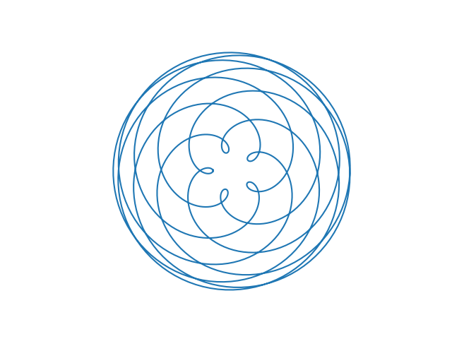
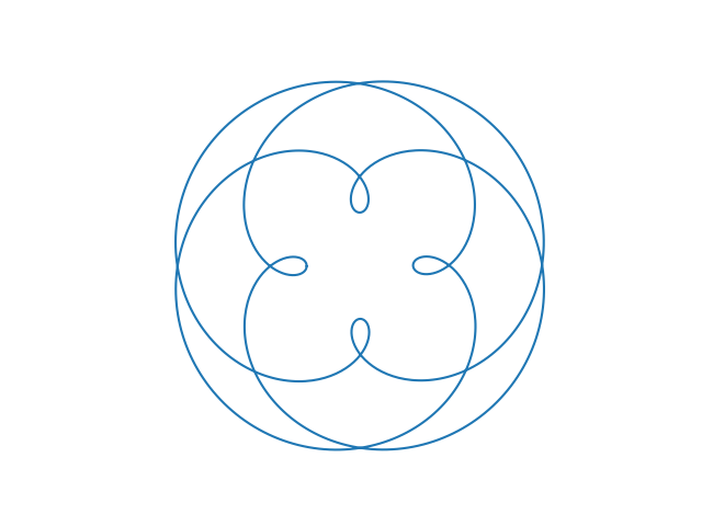
Jupiter / Saturn
The ratio of Saturn’s orbital period to that of Jupiter is nearly 5 to 2. If this ratio were exactly, the figure below would repeat itself every two Saturnine years. But the following plot is over 4 Saturnine years, showing that years 3 and 4 don’t exactly retrace the path of years 1 and 2.
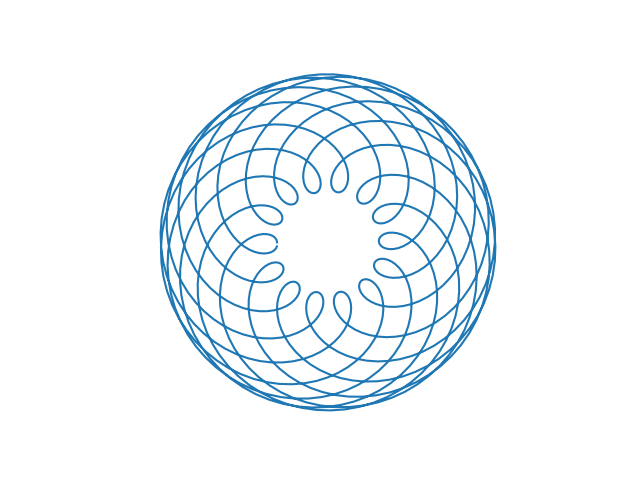
Uranus / Earth
Here’s what the orbit of Uranus looks like from Earth.
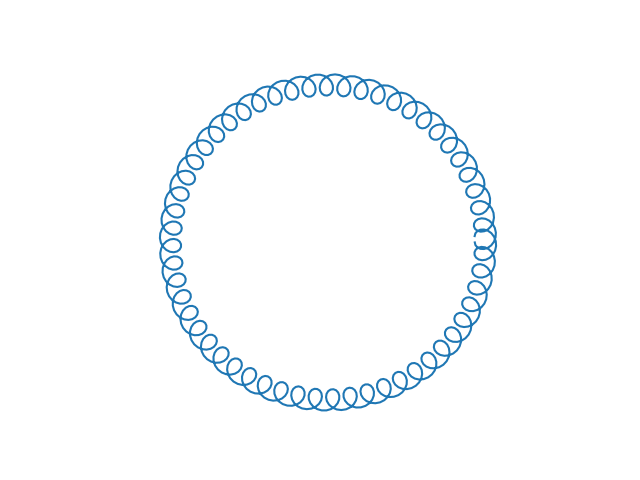
We see a big circle of tight little circles because the ratio of the distances from the sun is large.
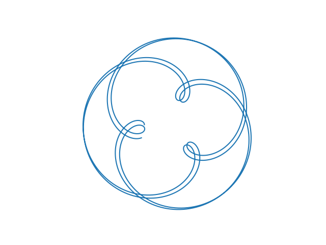
Mercury / Venus
Here’s what Mercury looks like from Venus.
Jovian moons
The same math that describes planets around the sun describes moons orbiting a planet. Here is what the orbit of Ganymede looks like from Callisto, and vice versa, as they orbit Jupiter. Ganymede completes 7 orbits in the time it takes Callisto to complete 3 orbits.
Python code
Here’s the code that produced the plots.
    import matplotlib.pyplot as plt
    from numpy import linspace, sin, cos, pi

    period = {
        'mercury' : 87.96926,
        'venus'   : 224.7008,
        'earth'   : 365.25636,
        'mars'    : 686.97959,
        'ceres'   : 1680.22107,
        'jupiter' : 4332.8201,
        'saturn'  : 10755.699,
        'uranus'  : 20687.153,
        'neptune' : 60190.03
    }

    dist = lambda T : T**(2/3) # Kepler

    def plot_orbit(planet1, planet2, periods=10):
        T1 = period[planet1]
        T2 = period[planet2]
        d1 = dist(T1)
        d2 = dist(T2)

        theta = linspace(0, 2*pi*periods, 1000)
        x = d1*cos(T2*theta/T1) - d2*cos(theta)
        y = d1*sin(T2*theta/T1) - d2*sin(theta)

        plt.gca().set_aspect("equal")
        plt.axis('off')
        plt.plot(x, y)
        plt.show()

    plot_orbit("venus", "earth", 8)
    plot_orbit("jupiter", "saturn", 4)
    plot_orbit("uranus", "earth", 57)
    plot_orbit("mercury", "venus", 9)