Cayley graphs in Mathematica

The previous post mentioned the group S4, the group of all permutations of a set with four elements. This post will show a way to visualize this group.

The Mathematica command

    CayleyGraph[
        SymmetricGroup[4], 
        VertexLabels -> Placed["Name", Center],
        VertexSize -> 0.4]

generates the graph below.

Cayley graph of alternating group S4

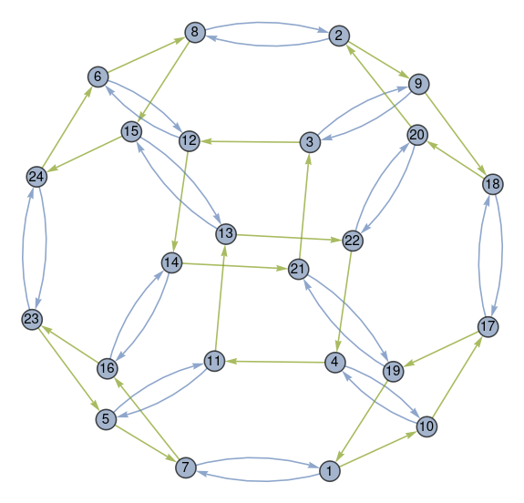
This is an interesting image, but what does it mean?

The elements of S4 are represented by the circled numbers. The numbers correspond to the permutations of four elements, listed in lexicographical order. If you label the four elements a, b, c, and d then the permutations are listed in alphabetical order. Permutation 1 is [1, 2, 3, 4] to itself and Permutation 24 is its reverse [4, 3, 2, 1].

In the Mathematica application, mousing over a number shows which permutation it represents, though the static image above doesn’t have this feature.

The blue arrows represent the permutation that swaps the first two elements. So the blue arrow between node 1 and node 7 says that swapping the first two elements of Permutation 1 gives you Permutation 7, which is [2, 1, 3, 4]. The blue arrow going back from 7 to 1 says that the same swapping operation applied to Permutation 7 returns you to Permutation 1.

All the blue arrows come in pairs because swapping is its own inverse.

The green arrows represent a rotation. For example, the green arrow from 1 to 10 says that rotation turns [1, 2, 3, 4] into [2, 3, 4, 1]. The rotation operation is not its own inverse, so the arrows only go in one direction. But every green arrow is part of a diamond because applying the rotation operation four times sends you back where you started.

You can get from any permutation to any other permutation by repeatedly either swapping the first two elements or applying a rotation. In group theoretical terminology, these two permutations generate the group S4.

Related posts

Permutations and centralizers in Mathematica

I had a fleeting thought about how little I use group theory when I realize I used it just this week.

A couple days ago I needed to know which permutations of 4 elements commute with reversal. If r takes a sequence and reverses it, I need to find all permutations p such that pr = rp.

In group theory jargon, the group of all permutations of 4 elements is the symmetric group S4. The subgroup of elements that commute with r is the centralizer of r. So my task was to find the centralizer of r in S4. How do I pose this task to Mathematica?

Mathematica represents permutations as disjoint cycles. The permutation r is represented as

    Cycles[{{4, 1}, {2, 3}}]

because swapping the first and last elements, then swapping the middle two elements, reverses a list of four elements.

To find the centralizer of r I asked Mathematica

    GroupCentralizer[SymmetricGroup[4], Cycles[{{4, 1}, {2, 3}}]]

This returns

    PermutationGroup[{Cycles[{{1, 4}}], Cycles[{{2, 3}}], Cycles[{{1, 2}, {3, 4}}]}]

This does list the permutations that commute with r but rather the generators of the group of such permutations. If we ask for the elements of the group above with

    GroupElements[%]

this returns

    {Cycles[{}], 
     Cycles[{{2, 3}}], 
     Cycles[{{1, 2}, {3, 4}}], 
     Cycles[{{1, 2, 4, 3}}], 
     Cycles[{{1, 3, 4, 2}}], 
     Cycles[{{1, 3}, {2, 4}}], 
     Cycles[{{1, 4}}], 
     Cycles[{{1, 4}, {2, 3}}]}

I use basic group theory and other algebra all the time, but I don’t think of it that way. In this example, I had a question about permutations, and it only occurred to me later that I could phrase my question in the vocabulary of group theory. I use ideas from algebra more often than I use the vocabulary of algebra.

Related posts

Floors and roots

I recently stumbled across the identity

\left\lfloor \sqrt{n} + \sqrt{n+1} + \sqrt{n+2}\right\rfloor = \left\lfloor \sqrt{9x+8}\right\rfloor

while reading [1]. Here ⌊x⌋ is the floor of x, the largest integer not larger than x.

My first thought was that this was hard to believe. Although the floor function is very simple, its interactions with other functions tends to be complicated. I was surprised that such a simple equation was true.

My second thought was that the equation makes sense. For large n the three terms on the left are roughly equal, and so

\sqrt{n} + \sqrt{n+1} + \sqrt{n+2} \approx 3 \sqrt{n+1} = \sqrt{9n + 9}

Not only that, the approximation gets better as n gets larger. So the theorem is at least plausible.

My third thought was that there is something subtle going on here. Why the 8 on the right hand side? It turns out the theorem is false if you replace the 8 with a 9. Equality fails to hold for n = 0, 3, 8, 15, …

There is a difference between saying xy and saying ⌊x⌋ = ⌊y⌋. The former makes the latter plausible, but it’s not the same. If x and y are very close, but on opposite sides of an integer, then ⌊x⌋ ≠ ⌊y⌋.

In fact, the approximation

\sqrt{n} + \sqrt{n+1} + \sqrt{n+2} \approx \sqrt{9n+a}

is better when a = 9 than when a = 8. Here’s a plot of the approximation errors.

So there’s something clever going on with the selection a = 8.

According to [1], the equation at the top was proposed as a problem in 1988 and a solution was published in 2005. The time span between the proposed theorem and its proof suggests that the proof isn’t trivial, though I have not yet read it.

This is an obscure problem, and so we can’t assume that hundreds of mathematicians were feverishly trying to find a solution for 17 years. On the other hand, if there were a trivial proof it seems someone would have posted it quickly.

[1] Prapanpong Pongsriiam. Analytic Number Theory for Beginners, 2nd edition.. American Mathematical Society 2023

Multiplication via parabola

Here’s a graphical way to multiply two positive numbers a and b using the parabola y = x².

  1. Start at the origin, move a units to the left, then go up vertically to the parabola, and draw a point.
  2. Go back to the origin, move b units to the right, go up vertically to the parabola, and draw another point.
  3. Connect the points and see where they cross the y-axis. That point is ab.

Here’s an example multiplying 3 and 5.

Multiplying numbers geometrically via a parabola

Here’s why this works. The slope of the line is the change in y over the change in x which is

m = (b² − a²)/(b − (−a)) = ba.

Use the equation of a line

yy0 = m(xx0)

with x0 = b and y0 = b² to get

y − b² = (ba)(xb).

Stick in x = 0 and you get y = ab.

Beta inequalities and cross ratios

When I worked at MD Anderson Cancer Center, we spent a lot of compute cycles evaluating the function g(a, b, c, d), defined as the probability that a sample from a beta(a, b) random variable is larger than a sample from a beta(c, d) random variable. This function was often in the inner loop of simulations that ran for hours or even days.

I developed ways to evaluate this function more efficiently because it was a bottleneck. Along the way I found a new symmetry. W. R. Thompson had studied what I call the function g back in 1933 and reported two symmetries:

g(a, b, c, d) = 1 − g(c, d, a, b)

and

g(a, b, c, d) = g(d, c, b, a).

I found that

g(a, b, c, d) = g(d, b, c, a)

as well. See a proof here.

You can conclude from these rules that

  1. g(a, b, c, d) = g(d, c, b, a) = g(d, b, c, a) = g(a, c, b, d)
  2. g(a, b, c, d) = 1 − g(c, d, a, b)

I was just looking at a book that mentioned the symmetries of the cross ratio which I will denote

r(a, b, c, d) = (ac)(b d) / (bc)(ad).

Here is Theorem 4.2 from [1] written in my notation.

Let a, b, c, d be four points on a projective line with cross ratio r(a, b, c, d) = λ. Then we have

    1. r(a, b, c, d) = r(b, a, d, c) = r(c, d, a, b) = r(d, c, b, a).
    2. r(a, b, d, c) = 1/λ
    3. r(a, c, b, d) = 1 − λ
    4. the values for the remaining permutations are consequences of these three basic rules.

This looks awfully familiar. Rules 1 and 3 for cross ratios correspond to rules 1 and 2 for beta inequalities, though not in the same order. Both g and r are invariant under reversing their arguments, but are otherwise invariant under different permutations of the arguments.

Both g and r take on 6 distinct values, taking on each 4 times. I feel like there is some deeper connection here but I can’t see it. Maybe I’ll come back to this later when I have the time to explore it. If you see something, please leave a comment.

There is no rule for beta inequalities analogous to rule 2 for cross ratios, at least not that I know of. I don’t know of any connection between g(a, b, c, d) and g(a, b, d, c).

Update: There cannot be a function h such that g(a, b, d, c) is a function of g(a, b, c, d) alone because I found parameters that lead to the same value of the latter but different values of the former. If there is a relation between g(a, b, c, d) and g(a, b, d, c) and it must involve the parameters and not just the value of g.

[1] Jürgen Richter-Gebert. Perspectives on Projective Geometry: A Guided Tour Through Real and Complex Geometry. Springer 2011.


The 10th Dedekind number

The nth Dedekind number M(n) is the number of monotone Boolean functions of n variables. The 9th Dedekind number was recently computed to be

M(9) = 286386577668298411128469151667598498812366.

The previous post defines monotone Boolean functions and explicitly enumerates the functions for one, two, or three variables. As that post demonstrates, M(1) = 3, M(2) = 6, and M(3) = 20. But as n increases, M(n) increases rapidly, with M(9) being on the order of 1041.

Although computing the Dedekind numbers exactly is difficult—M(8) was computed in 1991 and M(9) now in 2023—there is an explicit formula for these numbers, and much is known about their asymptotic growth. This post speculates about what M(10) might be.

Write the number k in binary and let bik be its ith bit:

b_i^k=\left\lfloor\frac{k}{2^i}\right\rfloor - 2\left\lfloor\frac{k}{2^{i+1}}\right\rfloor

Then the nth Dedekind number is given by

M(n)=\sum_{k=1}^{2^{2^n}} \prod_{j=1}^{2^n-1} \prod_{i=0}^{j-1} \left(1-b_i^k b_j^k\prod_{m=0}^{\log_2 i} (1-b_m^i+b_m^i b_m^j)\right)

and so

M(10)=\sum_{k=1}^{2^{1024}} \prod_{j=1}^{1023} \prod_{i=0}^{j-1} \left(1-b_i^k b_j^k\prod_{m=0}^{\log_2 i} (1-b_m^i+b_m^i b_m^j)\right)

In principle, all you have to do to compute M(10) is evaluate the sum above. However, since this sum has more than 10308 terms, it would take a while.

What can we say about M(10) without computing it? The number of monotone Boolean functions of n variables is less than the total number of Boolean functions of n variables, which equals

2^{2^n}

That tells us M(10) < 1.8 × 10308.

There are more useful bounds. It has been proven that

{n\choose \lfloor n/2\rfloor}\le \log_2 M(n)\le {n\choose \lfloor n/2\rfloor}\left(1+O\left(\frac{\log n}{n}\right)\right)

This gives us a definite lower bound but not a definite upper bound. We know M(10) ≥ 2252 which is approximately 7.237 × 1075, but we don’t know what the big-O term is. All we know is that for sufficiently large n, this term is smaller than some multiple of log(n)/n. How large does n need to be and what is this constant? I don’t know. Maybe researchers in this area have some partial results.

Let’s take a guess at the upper bound by seeing what the big-O term was for M(9). Find k such that

\log_2 M(9) = \binom{9}{4}\left(1 + k \frac{\log 9}{9}\right)

We get

k = \left(\frac{\log_2M(9)}{126} - 1 \right)\frac{9}{\log 9} \approx 0.3809

and we can use this to guess that

\log_2 M(10) \stackrel{?}{=} \binom{10}{5}\left(1 + 0.3809 \frac{\log 10}{10}\right) \approx 274.1

which would imply M(10) = 3.253 × 1082.

So to recap, we know for certain that M(10) is between 7.237 × 1075 and 1.8 × 10308, and our guess based on the heuristic above is that M(10) = 3.253 × 1082.

Enumerating monotone Boolean functions

The 9th Dedekind number was recently computed. What is a Dedekind number and why was it a big deal to compute just the 9th one of them?

We need to define a couple terms before we can define Dedekind numbers.

A Boolean function is a function whose inputs are 0’s and 1’s and whose output is 0 or 1.

A function f is monotone if increasing the input cannot decrease the output:

xyf(x) ≤ f(y).

Obviously a monotone Boolean function is a Boolean function that is monotone, but monotone with respect to what order? How are we to define when xy when x and y are sequences of bits?

There are numerous ways one might order the inputs, but the conventional order [1] in this context is to say x ≤ y if every bit in x is less than or equal to the corresponding bit in y. So if the ith bit of x is a 1, then the ith bit of y must be a 1.

A Boolean function is monotone if and only if flipping an input bit from 0 to 1 cannot change the output from 1 to 0.

Enumerating monotone Boolean functions

The nth Dedekind number M(n) is the number of monotone Boolean functions of n variables. We’ll enumerate a few of these. Let a, b, c and d be Boolean variables and denote AND by ∧ and OR by ∨. As usual, we assume ∧ is higher precedence than ∨ so that, for example,

xyz

means

x ∨ (yz).

One variable

There are three monotone functions of one variable a: always return 0, always return a, and always return 1.

  • 0
  • a
  • 1

The only Boolean function of one variable that isn’t monotone is the function that flips a, i.e. f(a) = ¬a.

Two variables

There are six monotone Boolean functions with two variables:

  • 0
  • a
  • b
  • a ∧ b
  • a ∨ b
  • 1

and so M(2) = 6.

We can verify that the six functions above are monotone with the following Python code.

    from itertools import product
    
    f = [None]*6
    f[0] = lambda a, b: 0
    f[1] = lambda a, b: a
    f[2] = lambda a, b: b
    f[3] = lambda a, b: a | b 
    f[4] = lambda a, b: a & b
    f[5] = lambda a, b: 1
    
    for i in range(6):
        for (a, b) in product((0,1), repeat=2):
            for (x, y) in product((0,1), repeat=2):
                if a <= x and b <= y:
                    assert(f[i](a, b) <= f[i](x, y))

Three variables

There are 20 monotone Boolean functions of three variables:

  • 0
  • a
  • b
  • c
  • a ∧ b
  • bc
  • ac
  • ab
  • bc
  • ac
  • abc
  • bca
  • acb
  • abbc
  • acbc
  • abac
  • abbcac
  • abc
  • abc

and so M(3) = 20.

As before, we can verify that the functions above are monotone with a script.

    g = [None]*20
    g[ 0] = lambda a, b, c: 0
    g[ 1] = lambda a, b, c: a 
    g[ 2] = lambda a, b, c: b
    g[ 3] = lambda a, b, c: c
    g[ 4] = lambda a, b, c: a & b
    g[ 5] = lambda a, b, c: b & c
    g[ 6] = lambda a, b, c: a & c
    g[ 7] = lambda a, b, c: a | b
    g[ 8] = lambda a, b, c: b | c
    g[ 9] = lambda a, b, c: a | c
    g[10] = lambda a, b, c: a & b | c
    g[11] = lambda a, b, c: b & c | a
    g[12] = lambda a, b, c: a & c | b
    g[13] = lambda a, b, c: a & b | b & c
    g[14] = lambda a, b, c: a & c | b & c
    g[15] = lambda a, b, c: a & b | a & c
    g[16] = lambda a, b, c: a & b | b & c | a & c
    g[17] = lambda a, b, c: a & b & c
    g[18] = lambda a, b, c: a | b | c 
    g[19] = lambda a, b, c: 1
    
    for i in range(20):
        for (a, b, c) in product((0,1), repeat=3):
            for (x, y, z) in product((0,1), repeat=3):
                if a <= x and b <= y and c <= z:
                    assert(g[i](a, b, c) <= g[i](x, y, z))

More variables

The concrete approach to enumerating monotone Boolean functions does not scale. There are 168 monotone functions of four variables, 7581 of five variables, and 7,828,354 functions of six variables. The Dedekind numbers M(n) grow very quickly. The next post will quantify just how quickly.


[1] This “order” is technically a partial order. If x = (0, 1) and y = (1, 0) then x and y are not comparable; neither is less than or equal to the other.

Drag equation exponent variation

The motion of a falling body of mass m is given by

m \frac{dv}{dt} = mg - kv^r

where the term −kvr accounts for drag due to air resistance. One can derive r = 2 under simple physical assumptions, but if I remember correctly other values of r may be more realistic in certain circumstances. I don’t know much about the physics here; if you know about the use of other values of r, please let me know by leaving a comment.

Terminal velocity

When r = 1 or r = 2 the differential equation above can be solved in terms of elementary functions, but otherwise it cannot. Nevertheless one can show that for all values of r the object reaches a terminal velocity, and calculate that velocity without explicitly solving the differential equation. William Waterhouse demonstrated this in a one-page article [1]. He rewrites the equation to look at time as a function of velocity rather than velocity as a function of time

\frac{dt}{dv} = \frac{1}{g} \frac{1}{1 - (k/mg)v^r}

and concludes

t = \frac{1}{g} \int_0^v \frac{dv}{1 - (k/mg)v^r} + t_0

He notes that the integral diverges as v approaches

 \left(\frac{mg}{k}\right)^{1/r}

and so that is the terminal velocity, i.e. it takes an infinite amount of time to achieve this velocity. Waterhouse recommends this derivation as “a good example of deriving information about a problem without knowing an explicit solution.”

I would add that such an approach is the norm, not an exception. A closed-form solution to a differential equation in nice when you can get it, but usually not possible. And even when you can find a closed-form solution, you may be able to achieve your goal more directly by not using it.

Hypergeometric solution

I suspected the differential equation could be solved for general values of r using special functions, and that is the case. Mathematica was able to evaluate the integral for t as a function of v in terms of a hypergeometric function.

v \, _2F_1\left(1,\frac{1}{r};1+\frac{1}{r};\frac{g k v^r}{m}\right)

When I asked Mathematica to solve the differential equation directly, it said that the solution is the inverse function of the function above. Apparently Waterhouse and Mathematica agree that it is easier to think of t as a function of v rather than the original formulation.

The notation 2F1 indicates there are two upper parameters and one lower parameter. In our application, the upper parameters are 1 and 1/r, the lower parameter is 1 + 1/r, and the function is evaluated at gkvr/m. You can find a brief introduction to hypergeometric functions here. A hypergeometric function 2F1 has a singularity at 1, and so we could derive the terminal velocity from the explicit solution.

Mathematica implementation

Let c = gk/m. Then we can express velocity as a function of time in Mathematica by

    f[r_, c_, v_] := InverseFunction
    [
        #1 Hypergeometric2F1[1, 1/r, 1 + 1/r, c #1^r] &
    ][t]

and use this to make plots of the velocity for various values of c and r.

The following sets c = 2 and varies r over 1, 1.1, 1.2, … 2.

    Plot[Table[f[2, d/10, t], {d, 10, 20}], {t, 0, 4}, PlotRange -> All]

Here’s the output.

The terminal velocity decreases as r increases. The opposite is true for c < 1.

[1] William C. Waterhouse. A Fact about Falling Bodies. Mathematics Magazine, Vol. 44, No. 1 (Jan., 1971), pp. 33–34. The article straddles two pages, but takes up less than half of each page.

Numbers don’t typically have many prime factors

Suppose you select a 100-digit number at random. How many distinct prime factors do you think it would have?

The answer is smaller than you might think: most likely between 5 and 6.

The function ω(n) returns the number of distinct prime factors of n [1]. A theorem of Hardy and Ramanujan says that as N goes to infinity, the average value of ω(n) for positive integers up to N is log log N.

Since log log 10100 = 5.43…, we’d expect 100-digit numbers to have between 5 and 6 distinct factors.

The above calculation gives the average number of distinct prime factors for all numbers with up to 100 digits. But if we redid the calculation looking at numbers between 1099 and 10100 it would only make a difference in the third decimal place.

Let’s look at a much smaller example where we can tally the values of ω(n), numbers from 2 to 1,000,000.

Most numbers with up to six digits have two or three distinct prime factors, which is consistent with log log 106 ≈ 2.6.

There are 2,285 six-digit numbers that have six distinct prime factors. Because this is out of a million numbers, it corresponds to a bar in the graph above that is barely visible.

There are 8 six-digit number with 7 distinct prime factors and none with more factors.

Hardy’s theorem with Ramanujan established the mean of ω(n) for large numbers. The Erdős–Kac theorem goes further and says roughly that ω(n) is normally distributed with mean and variance log log n. More on this here.

So returning to our example of 100-digit numbers, the Hardy-Ramanujan theorem implies these numbers would have between 5 and 6 prime factors on average, and the Erdős–Kac theorem implies that about 95% of such numbers have 10 or fewer distinct prime factors. The maximum number of distinct prime factors is 54.

Related posts

[1] SymPy has a function primeomega, but it does not compute ω(n). Instead, it computes Ω(n), the number of prime factors of n counted with multiplicity. So, for example, ω(12) = 2 but Ω(12) = 3. The SymPy function to compute ω(n) is called primenu.

Every factorial is a power

The previous post mentioned that 24! ≈ 1024 and 25! ≈ 1025.

For every n, there is some base b such that n! = bn. For example, 30! ≈ 1230.

It’s easy to find b [1]:

b = \exp\left( \frac{\log n!}{n} \right)

What’s interesting is that b is very nearly a linear function of n.

In hindsight it’s clear that this should be the case—it follows easily from Stirling’s approximation—but I didn’t anticipate this before I plotted it.

Now fix n and find b such that n! = bn. Since the relationship between n and b(n) is nearly linear, this suggests

(2n)! \approx (2b)^{2n} = 2^{2n} (n!)^2

which is true. It follows from the multiplication identity for the gamma function:

Let z = n + 1/2 so that the left side is (2n)!. On the right side, Γ(z + 1/2) = n! and Γ(z) is not too different from n!. The rest of the right side is 22n/√π.

So our observation that b(n) is nearly linear gave us a hint of Gauss’s multiplication formula.

[1] Numerically you would probably evaluate this function by calling a routine that computes log Γ(n + 1) directly without computing Γ(n + 1) first. This avoids overflow for large n.

This is why mathematical libraries will have not only gamma functions but also loggamma functions. The latter seems redundant, but it’s not.