Converting very long strings to integers in Python

In the process of writing the previous post, I wanted to confirm that the number in the post

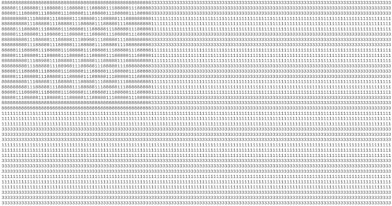
really is prime. This was useful in debugging my manual conversion of the image to text: errors did not result in a prime number. For example, I didn’t see the 9’s in the image at first, and I didn’t get a prime number until I changed four of the 8’s to 9’s.

But there was a problem along the way. Simply converting the string to an integer didn’t work. It produced the following error:

SyntaxError: Exceeds the limit (4300) for integer string conversion: value has 5382 digits; use sys.set_int_max_str_digits() to increase the limit – Consider hexadecimal for huge integer literals to avoid decimal conversion limits.

Note that the limitation is not on the size of a Python integer. The only limitation on the size of an integer is available memory. But there is a limitation on the size of string that can be converted to an integer.

The fix suggested in the error message didn’t work. But storing the number as several strings, i.e. each row of the image, and doing my own radix conversion did work.

from sympy import isprime

flaglines = [
    "888888888888888888888888888888888888888888888888888883333333333333333333333333333333333333333333333333333333333333333333333333333333333333",
    "888881118888811188888111888881118888811188888111888883333333333333333333333333333333333333333333333333333333333333333333333333333333333333",
    "888881118888811188888111888881118888811188888111888883333333333333333333333333333333333333333333333333333333333333333333333333333333333333",
    "888888888111888881118888811188888111888881118888888881111111111111111111111111111111111111111111111111111111111111111111111111111111111111",
    "888888888111888881118888811188888111888881118888888881111111111111111111111111111111111111111111111111111111111111111111111111111111111111",
    "888881118888811188888111888881118888811188888111888881111111111111111111111111111111111111111111111111111111111111111111111111111111111111",
    "888881118888811188888111888881118888811188888111888883333333333333333333333333333333333333333333333333333333333333333333333333333333333333",
    "888888888111888881118888811188988111888881118888888883333333333333333333333333333333333333333333333333333333333333333333333333333333333333",
    "888888888111888881118898811188888111888881118888888883333333333333333333333333333333333333333333333333333333333333333333333333333333333333",
    "888881118888811188888111888881118888811188888111888881111111111111111111111111111111111111111111111111111111111111111111111111111111111111",
    "888881118888811188888111888881118888811188888111888881111111111111111111111111111111111111111111111111111111111111111111111111111111111111",
    "888888888111889881118888811188888111888881118888888881111111111111111111111111111111111111111111111111111111111111111111111111111111111111",
    "888888888111888881118898811188888111888881118888888883333333333333333333333333333333333333333333333333333333333333333333333333333333333333",
    "888881118888811188888111888881118888811188888111888883333333333333333333333333333333333333333333333333333333333333333333333333333333333333",
    "888881118888811188888111888881118888811188888111888883333333333333333333333333333333333333333333333333333333333333333333333333333333333333",
    "888888888111888881118888811188888111888881118888888881111111111111111111111111111111111111111111111111111111111111111111111111111111111111",
    "888888888111888881118888811188888111888881118888888881111111111111111111111111111111111111111111111111111111111111111111111111111111111111",
    "888881118888811188888111888881118888811188888111888881111111111111111111111111111111111111111111111111111111111111111111111111111111111111",
    "888881118888811188888111888881118888811188888111888883333333333333333333333333333333333333333333333333333333333333333333333333333333333333",
    "888888888888888888888888888888888888888888888888888883333333333333333333333333333333333333333333333333333333333333333333333333333333333333",
    "888888888888888888888888888888888888888888888888888883333333333333333333333333333333333333333333333333333333333333333333333333333333333333",
    "111111111111111111111111111111111111111111111111111111111111111111111111111111111111111111111111111111111111111111111111111111111111111111",
    "111111111111111111111111111111111111111111111111111111111111111111111111111111111111111111111111111111111111111111111111111111111111111111",
    "111111111111111111111111111111111111111111111111111111111111111111111111111111111111111111111111111111111111111111111111111111111111111111",
    "333333333333333333333333333333333333333333333333333333333333333333333333333333333333333333333333333333333333333333333333333333333333333333",
    "333333333333333333333333333333333333333333333333333333333333333333333333333333333333333333333333333333333333333333333333333333333333333333",
    "333333333333333333333333333333333333333333333333333333333333333333333333333333333333333333333333333333333333333333333333333333333333333333",
    "111111111111111111111111111111111111111111111111111111111111111111111111111111111111111111111111111111111111111111111111111111111111111111",
    "111111111111111111111111111111111111111111111111111111111111111111111111111111111111111111111111111111111111111111111111111111111111111111",
    "111111111111111111111111111111111111111111111111111111111111111111111111111111111111111111111111111111111111111111111111111111111111111111",
    "333333333333333333333333333333333333333333333333333333333333333333333333333333333333333333333333333333333333333333333333333333333333333333",
    "333333333333333333333333333333333333333333333333333333333333333333333333333333333333333333333333333333333333333333333333333333333333333333",
    "333333333333333333333333333333333333333333333333333333333333333333333333333333333333333333333333333333333333333333333333333333333333333333",
    "111111111111111111111111111111111111111111111111111111111111111111111111111111111111111111111111111111111111111111111111111111111111111111",
    "111111111111111111111111111111111111111111111111111111111111111111111111111111111111111111111111111111111111111111111111111111111111111111",
    "111111111111111111111111111111111111111111111111111111111111111111111111111111111111111111111111111111111111111111111111111111111111111111",
    "333333333333333333333333333333333333333333333333333333333333333333333333333333333333333333333333333333333333333333333333333333333333333333",
    "333333333333333333333333333333333333333333333333333333333333333333333333333333333333333333333333333333333333333333333333333333333333333333",
    "333333333333333333333333333333333333333333333333333333333333333333333333333333333333333333333333333333333333333333333333333333333333333333",
]

m = int(flaglines[0])
for i in range(1, len(flaglines)):
    line = flaglines[i]
    x = int(line)
    m = m * 10**len(line) + x
print(isprime(n))

Monero’s elliptic curve

Monero logo
Digital signatures often use elliptic curves. For example, Bitcoin and Ethereum use the elliptic curve secp256k1 [1]. This post will discuss the elliptic curve Ed25519 [2] using in Monero and in many other applications.

Ed25519 has the equation

y² − x² = 1 + d x² y²

over the finite field Fq where q = 2255 − 19 and d = −121665/121666. The general form of the equation above makes Ed25519 a “twisted Edwards curve.”

The expression for d is not the rational number it appears to be. Think of it as

d = −121665 × 121666−1

where the multiplication and the multiplicative inverse are calculated mod q.

We could calculate d in Python as follows.

>>> q = 2**255 - 19
>>> d = (-121665*pow(121666, -1, q)) % q
>>> d 
37095705934669439343138083508754565189542113879843219016388785533085940283555

The equation above does not look like an elliptic curve if you think of an elliptic curve having the form

y² = x³ + ax + b.

But that form, known as Weierstrass form, is not the most general definition of an elliptic curve. Elliptic curves can be written in that form [3] but they do not have to be. There are computational advantages to writing curves in the form

y² − x² = 1 + d x² y²

when possible rather than in Weierstrass form [4].

Elliptic curve digital signatures require a specified base point. The Monero whitepaper describes the base point simply as

G = (x, −4/5).

That’s leaving out a fair bit of detail. First of all, 4/5 is interpreted as 4 times the multiplicative inverse of 5 mod q, similar to the calculation for d above.

>>> y = (-4*pow(5, -1, q)) % q; y
11579208923731619542357098500868790785326998466564056403945758400791312963989

Now we have two tasks. How do we solve for x, and which solution do we take?

We need to solve

x² = (y² − 1)/(1 + d y²) mod q.

We can do this in Python as follows.

>>> from sympy import sqrt_mod
>>> roots = sqrt_mod((y**2 - 1)*pow(1 + d*y**2, -1, q), q, all_roots=True)
>>> roots 
[15112221349535400772501151409588531511454012693041857206046113283949847762202,
42783823269122696939284341094755422415180979639778424813682678720006717057747]

So which root to we choose? The convention is to use the even solution, the first one above. (The two roots add to 0 mod q; one will be odd and one will be even because q is odd.)

We can verify that (x, y) is on the Ed25519 elliptic curve:

>>> ((y**2 - x**2) - (1 + d*x**2 * y**2)) % q
0

Related posts

[1] The name secp256k1 was created as follows. The “sec” comes from “Standards for Efficient Cryptography,” referring to the group that specified the curve parameters. The “p” means the curve is over a finite field of prime order. The order of the curve is slightly less than 2256. The “k” indicates that this is a Koblitz curve.

[2] The “Ed” part of the name refers to Harold Edwards, the mathematician who studied the family of elliptic curves now known as Edwards curves. The “25519” part of the name refers to the fact that the curve is over the finite field with 2255 − 19 elements.

[3] Provided the elliptic curve is not over a field of characteristic 2 or 3.

[4] Group operations can be implemented more efficiently and the point at infinity can be handled without exception logic.

Converting between quaternions and rotation matrices

In the previous post I wrote about representing rotations with quaternions. This representation has several advantages, such as making it clear how rotations compose. Rotations are often represented as matrices, and so it’s useful to be able to go between the two representations.

A unit-length quaternion (q0, q1, q2, q3) represents a rotation by an angle θ around an axis in the direction of (q1, q2, q3) where cos(θ/2) = q0. The corresponding rotation matrix is given below.

R = \begin{pmatrix} 2(q_0^2 + q_1^2) - 1 & 2(q_1 q_2 - q_0 q_3) & 2(q_1 q_3 + q_0 q_2) \\ 2(q_1 q_2 + q_0 q_3) & 2(q_0^2 + q_2^2) - 1 & 2(q_1 q_3 - q_0 q_1) \\ 2(q_1 q_3 - q_0 q_2) & 2(q_2 q_3 + q_0 q_1) & 2(q_0^2 + q_3^2) - 1 \end{pmatrix}

Going the other way around, inferring a quaternion representation from a rotation matrix, is harder. Here is a mathematically correct but numerically suboptimal method known [1] as the Chiaverini-Siciliano method.

\begin{align*} q_0 &= \frac{1}{2} \sqrt{1 + r_{11} + r_{22} + r_{33}} \\ q_1 &= \frac{1}{2} \sqrt{1 + r_{11} - r_{22} - r_{33}} \text{ sgn}(r_{32} - r_{32}) \\ q_2 &= \frac{1}{2} \sqrt{1 - r_{11} + r_{22} - r_{33}} \text{ sgn}(r_{13} - r_{31}) \\ q_3 &= \frac{1}{2} \sqrt{1 - r_{11} - r_{22} + r_{33}} \text{ sgn}(r_{21} - r_{12}) \end{align*}

Here sgn is the sign function; sgn(x) equals 1 if x is positive and −1 if x is negative. Note that the components only depend on the diagonal of the rotation matrix, aside from the sign terms. Better numerical algorithms make more use of the off-diagonal elements.

Accounting for degrees of freedom

Something seems a little suspicious here. Quaternions contain four real numbers, and 3 by 3 matrices contain nine. How can four numbers determine nine numbers? And going the other way, out of the nine, we essentially choose three that determine the four components of a quaternion.

Quaternions have four degrees of freedom, but we’re using unit quaternions, so there are basically three degrees of freedom. Likewise orthogonal matrices have three degrees of freedom. An axis of rotation is a point on a sphere, so that has two degrees of freedom, and the degree of rotation is the third degree of freedom.

In topological terms, the unit quaternions and the set of 3 by 3 orthogonal matrices are both three dimensional manifolds, and the former is a double cover of the latter. It is a double cover because a unit quaternion q corresponds to the same rotation as −q.

Python code

Implementing the equations above is straightforward.

import numpy as np

def quaternion_to_rotation_matrix(q):
    q0, q1, q2, q3 = q
    return np.array([
        [2*(q0**2 + q1**2) - 1, 2*(q1*q2 - q0*q3), 2*(q1*q3 + q0*q2)],
        [2*(q1*q2 + q0*q3), 2*(q0**2 + q2**2) - 1, 2*(q2*q3 - q0*q1)],
        [2*(q1*q3 - q0*q2), 2*(q2*q3 + q0*q1), 2*(q0**2 + q3**2) - 1]
    ]) 

def rotation_matrix_to_quaternion(R):
    r11, r12, r13 = R[0, 0], R[0, 1], R[0, 2]
    r21, r22, r23 = R[1, 0], R[1, 1], R[1, 2]
    r31, r32, r33 = R[2, 0], R[2, 1], R[2, 2]
    
    # Calculate quaternion components
    q0 = 0.5 * np.sqrt(1 + r11 + r22 + r33)
    q1 = 0.5 * np.sqrt(1 + r11 - r22 - r33) * np.sign(r32 - r23)
    q2 = 0.5 * np.sqrt(1 - r11 + r22 - r33) * np.sign(r13 - r31)
    q3 = 0.5 * np.sqrt(1 - r11 - r22 + r33) * np.sign(r21 - r12)
    
    return np.array([q0, q1, q2, q3])

Random testing

We’d like to test the code above by generating random quaternions, converting the quaternions to rotation matrices, then back to quaternions to verify that the round trip puts us back essentially where we started. Then we’d like to go the other way around, starting with randomly generated rotation matrices.

To generate a random unit quaternion, we generate a vector of four independent normal random values, then normalize by dividing by its length. (See this recent post.)

To generate a random rotation matrix, we use a generator that is part of SciPy.

Here’s the test code:

def randomq():
    q = norm.rvs(size=4)
    return q/np.linalg.norm(q)

def randomR():
    return special_ortho_group.rvs(dim=3)

np.random.seed(20250507)
N = 10

for _ in range(N):
    q = randomq()
    R = quaternion_to_rotation_matrix(q)
    t = rotation_matrix_to_quaternion(R)
    print(np.linalg.norm(q - t))
    
for _ in range(N):
    R = randomR()
    q = rotation_matrix_to_quaternion(R)
    T = quaternion_to_rotation_matrix(q)
    print(np.linalg.norm(R - T))

The first test utterly fails, returning six 2s, i.e. the round trip vector is as far as possible from the vector we started with. How could that happen? It must be returning the negative of the original vector. Now go back to the discussion above about double covers: q and −q correspond to the same rotation.

If we go back and add the line

    q *= np.sign(q[0])

then we standardize our random vectors to have a positive first component, just like the vectors returned by rotation_matrix_to_quaternion.

Now our tests all return norms on the order of 10−16 to 10−14. There’s a little room to improve the accuracy, but the results are good.

Update: I did some more random testing, and found errors on the order of 10−10. Then I was able to create a test case where rotation_matrix_to_quaternion threw an exception because one of the square roots had a negative argument. In [1] the authors get around this problem by evaluating two theoretically equivalent expressions for each of the square root arguments. The expressions are complementary in the sense that both should not lead to numerical difficulties at the same time.

[1] See “Accurate Computation of Quaternions from Rotation Matrices” by Soheil Sarabandi and Federico Thomas for a better numerical algorithm. See also the article “A Survey on the Computation of Quaternions From Rotation Matrices” by the same authors.

How hard is constraint programming?

I’ve been writing code for the Z3 SMT solver for several months now. Here are my findings.

Python is used here as the base language. Python/Z3 feels like a two-layer programming model—declarative code for Z3, imperative code for Python. In this it seems reminiscent of C++/CUDA programming for NVIDIA GPUs—in that case, mixed CPU and GPU imperative code. Either case is a clever combination of methodologies that is surprisingly fluent and versatile, albeit not a perfect blend of seamless conceptual cohesion.

Other comparisons:

  • Both have two separate memory spaces (CUDA CPU/GPU memories for one; pure Python variables and Z3 variables for the other).
  • Both can be tricky to debug. In earlier days, CUDA had no debugger, so one had to fall back to the trusty “printf” statement (for a while it didn’t even have that!). If the code crashed, you might get no output at all. To my knowledge, Z3 has no dedicated debugger. If the problem being solved comes back as satisfiable, you can print out the discovered model variables, but if satisfiability fails, you get very little information. Like some other novel platforms, something of a “black box.”
  • In both cases, programmer productivity can be well-served by developing custom abstractions. I developed a Python class to manage multidimensional arrays of Z3 variables, this was a huge time saver.

There are differences too, of course.

  • In Python, “=” is assignment, but in Z3, one only has “==”, logical or numeric equality, not assignment per se. Variables are set once and can’t be changed—sort of a “write-once variables” programming model—as is natural to logic programming.
  • Code speed optimization is challenging. Code modifications for Z3 constraints/variables can have extreme and unpredictable runtime effects, so it’s hard to optimize. Z3 is solving an NP-complete problem after all, so runtimes can theoretically increase massively. Speedups can be massive also; one round of changes I made gave 2000X speedup on a test problem. Runtime of CUDA code can be unpredictable to a lesser degree, depending on the PTX and SASS code generation phases and the aggressive code optimizations of the CUDA compiler. However, it seems easier to “see through” CUDA code, down to the metal, to understand expected performance, at least for smaller code fragments. The Z3 solver can output statistics of the solve, but these are hard to actionably interpret for a non-expert.
  • Z3 provides many, many algorithmic tuning parameters (“tactics”), though it’s hard to reason about which ones to pick. Autotuners like FastSMT might help. Also there have been some efforts to develop tools to visualize the solve process, this might be of help.

It would be great to see more modern tooling support and development of community best practices to help support Z3 code developers.

Factored random numbers

A couple days ago Michael Nielsen posted an image of a one-page paper that gives an algorithm for generating factored random numbers, uniformly distributed from 1 to some designated N.

The algorithm does not generate random numbers then factor them. It’s more efficient than that, generating the factorization along with the final result. It does require testing for whether a number is prime, but this is more efficient than factorization.

I thought about trying to code up the algorithm in Python, but then I see that @iconjack beat me to it.

from sympy import isprime
from random import random, randint

def randfacts(N):
    while True:
        n, r, s = N, 1, []
        while n > 1:
            if r > N: break
            if isprime(n := randint(1,n)):
                r *= n
                s.append(n)
        else:
            if random() < r/N:
                return r, s

Python code for means

The last couple article have looked at various kinds of mean. The Python code for four of these means is trivial:

gm  = lambda a, b: (a*b)**0.5
am  = lambda a, b: (a + b)/2
hm  = lambda a, b: 2*a*b/(a+b)
chm = lambda a, b: (a**2 + b**2)/(a + b)

But the arithmetic-geometric mean (AGM) is not trivial:

from numpy import pi
from scipy.special import ellipk

agm = lambda a, b: 0.25*pi*(a + b)/ellipk((a - b)**2/(a + b)**2) 

The arithmetic-geometric mean is defined by iterating the arithmetic and geometric means and taking the limit. This iteration converges very quickly, and so writing code that directly implements the definition is efficient.

But the AGM can also be computed via a special function K, the “complete elliptic integral of the first kind,” which makes the code above more compact. This is conceptually nice because we can think of the AGM as a simple function, not an iterative process.

But how is K evaluated? In some sense it doesn’t matter: it’s encapsulated in the SciPy library. But someone has to write SciPy. I haven’t looked at the SciPy source code, but usually K is calculated numerically using the AGM because, as we said above, the AGM converges very quickly.

Bell curve meme: How to calculate the AGM? The left and right tails say to use a while loop. The middle says to evaluate a complete ellliptic integral of the first kind.

This fits the pattern of a bell curve meme: the novice and expert approaches are the same, but for different reasons. The novice uses an iterative approach because that directly implements the definition. The expert knows about the elliptic integral, but also knows that the iterative approach suggested by the definition is remarkably efficient and eliminates the need to import a library.

Although it’s easy to implement the AGM with a while loop, the code above does have some advantages. For one thing, it pushes the responsibility for validation and exception handling onto the library. On the other hand, the code is easy to get wrong because there are two conventions on how to parameterize K and you have to be sure to use the same one your library uses.

Searching for proper nouns

Suppose you want to find all the proper nouns in a document. You could grep for every word that starts with a capital letter with something like

    grep '\b[A-Z]\w+'

but this would return the first word of each sentence in addition to the words you’re after.

You could grep for capitalized words that are not preceded by a period or question mark followed by a space.

    grep -P '(?<![.?] )\b[A-Z]\w+'

That’s possibly better, but it misses proper nouns at the beginning of a sentence.

You might be able to accomplish what you’re after by tinkering with regular expressions, but it would be better to use a library that has some idea of what a proper noun is.

NLP with spaCy

The Python natural language processing library spaCy classifies words by part of speech, and so could in particular search for proper nouns.

Here’s an example using the opening lines of Moby Dick.

    import spacy
    nlp = spacy.load("en_core_web_lg")

    doc = nlp("Call me Ishmael. Some years ago—never mind how long precisely—having little or no money in my purse, and nothing particular to interest me on shore, I thought I would sail about a little and see the watery part of the world. Whenever I find myself growing grim about the mouth; whenever it is a damp, drizzly November in my soul ... I account it high time to get to sea as soon as I can.")

    for tok in doc:
        if tok.pos_ == "PROPN":
            print(tok)

This will print Ishmael and November only. It does not print words at the beginning of a sentence such as Call or Some even though they are capitalized. When spaCy got to the line

Queequeg was George Washington cannibalistically developed.

it detected that Queequeg is a proper noun. Presumably the model can tell this from context, because the word precedes the verb was and not because it knows Queequeg is proper name.

When I changed November to november spaCy was still able to detect that november was a proper noun. When I downcased Ishmael it did not detect that ishmael was a proper noun, presumably because Ishmael is an uncommon name. When I changed the text to “Call me tim” the library did recognize tim as a proper noun.

When I fed spaCy the sentence

I never go as a passenger; nor, though I am something of a salt, do I ever go to sea as a Commodore, or a Captain, or a Cook.

the library thought that Commodore, Captain, and Cook were proper nouns. If I downcase these words, spaCy does not flag them as proper nouns.

When processing the line

For as in this world,head winds are far more prevalent than winds from astern (that is, if you never violate the Pythagorean maxim), so for the most part the Commodore on the quarter-deck gets his atmosphere at second hand from the sailors on the forecastle

spaCy correctly flagged Commodore as a proper noun in this instance. Also, it did not classify Pythagorean as a proper noun; the word is proper but not a noun, i.e. it’s a proper adjective.

TANSTAAFL

My script above has only six lines of code. But it depends on a library that uses a 588 MB language model. [1]

Related posts

[1] “TANSTAALF” stands for “There ain’t no such thing as a free lunch.” It comes from The Moon is a Harsh Mistress by Heinlein.

Incidentally, when I fed “The term TANSTAAFL comes from The Moon is a Harsh Mistress by Heinlein.” to spaCy, it flagged Harsh and Mistress as proper nouns.

When I fed it “The term TANSTAAFL comes from ‘The moon is a harsh mistress’ by Heinlein.” the library correctly tagged harsh as an adjective and mistress as a (non-proper) noun.

Golden integration

Let φ be the golden ratio. The fractional parts of nφ bounce around in the unit interval in a sort of random way. Technically, the sequence is quasi-random.

Quasi-random sequences are like random sequences but better in the sense that they explore a space more efficiently than random sequences. For this reason, Monte Carlo integration (“integration by darts“) can often be made more efficient by replacing random sequences with quasi-random sequence. This post will illustrate this efficiency advantage in one dimension using the fractional parts of nφ.

Here are functions that will generate our integration points.

    from numpy import random, zeros

    def golden_source(n):
        phi = (1 + 5**0.5)/2
        return (phi*n)%1

    def random_source(N):
        return random.random()

We will pass both of these generators as arguments to the following function which saves a running average of function evaluates at the generated points.

    def integrator(f, source, N):
        runs = zeros(N)
        runs[0] = f(source(0))
        for n in range(1, N):
            runs[n] = runs[n-1] + (f(source(n)) - runs[n-1])/n
        return runs

We’ll use as our example integrand f(x) = x² (1 − x)³. The integral of this function over the unit interval is 1/60.

    def f(x):
        return x**2 * (1-x)**3
    exact = 1/60

Now we call our integrator.

    random.seed(20230429)
    N = 1000
    golden_run = integrator(f, golden_source, N)
    random_run = integrator(f, random_source, N)

Now we plot the difference between each run and the exact value of the integral. Both methods start out with wild fluctuations. We leave out the first 10 elements in order to make the error easier to see.

    import matplotlib.pyplot as plt

    k = 10
    x = range(N)
    plt.plot(x[k:], golden_run[k:] - exact)
    plt.plot(x[k:], random_run[k:] - exact)

This produces the following plot.

The integration error using φn − ⌊φn⌋ is so close to zero that it’s hard to observe its progress. So we plot it again, this time taking the absolute value of the integration error and plotting on a log scale.

    plt.plot(x[k:], abs(golden_run[k:] - exact))
    plt.plot(x[k:], abs(random_run[k:] - exact))
    plt.yscale("log")

This produces a more informative plot.

The integration error for the golden sequence is at least an order of magnitude smaller, and often a few orders of magnitude smaller.

The function we’ve integrated has a couple features that make integration using quasi-random sequences (QMC, quasi-Monte Carlo) more efficient. First, it’s smooth. If the integrand is jagged, QMC has no advantage over MC. Second, our integrand could be extended smoothly to a periodic function, i.e. f(0) = f(1) and f′(0) = f′(1). This makes QMC integration even more efficient.

Related posts

Python code to solve Kepler’s equation

The previous post looked at solving Kepler’s equation using Newton’s method. The problem with using Newton’s method is that it may not converge when the eccentricity e is large unless you start very close to the solution. As discussed at the end of that post, John Machin came up with a clever way to start close. His starting point is defined as follow.

\begin{align*} n &= \sqrt{5 + \sqrt{16 + \frac{9}{e}}} \\ M &= n \left((1-e)s + \frac{e(n^2 - 1) + 1}{6}s^3 \right) \\ x_0 &= n \arcsin s \end{align*}

The variable s is implicitly defined as the root of a cubic polynomial. This could be messy. Maybe there are three real roots and we have to decide which one to use. Fortunately this isn’t the case.

The discriminant of our cubic equation is negative, so there is only one real root. And because our cubic equation for s has no s² term the expression for the root isn’t too complicated.

Here’s Python code to solve Kepler’s equation using Newton’s method with Machin’s starting point.

    from numpy import sqrt, cbrt, pi, sin, cos, arcsin, random
    
    # This will solve the special form of the cubic we need.
    def solve_cubic(a, c, d):
        assert(a > 0 and c > 0)
        p = c/a
        q = d/a
        k = sqrt( q**2/4 + p**3/27 )
        return cbrt(-q/2 - k) + cbrt(-q/2 + k)
    
    # Machin's starting point for Newton's method
    # See johndcook.com/blog/2022/11/01/kepler-newton/
    def machin(e, M):
        n = sqrt(5 + sqrt(16 + 9/e))
        a = n*(e*(n**2 - 1)+1)/6
        c = n*(1-e)
        d = -M
        s = solve_cubic(a, c, d)
        return n*arcsin(s)    
    
    def solve_kepler(e, M):
        "Find E such that M = E - e sin E."
        assert(0 <= e < 1)
        assert(0 <= M <= pi) 
        f = lambda E: E - e*sin(E) - M 
        E = machin(e, M) 
        tolerance = 1e-10 

        # Newton's method 
        while (abs(f(E)) > tolerance):
            E -= f(E)/(1 - e*cos(E))
        return E

To test this code, we’ll generate a million random values of e and M, solve for the corresponding value of E, and verify that the solution satisfies Kepler’s equation.

    random.seed(20221102)
    N = 1_000_000
    e = random.random(N)
    M = random.random(N)*pi
    for i in range(N):
        E = solve_kepler(e[i], M[i])
        k = E - e[i]*sin(E) - M[i]
        assert(abs(k) < 1e-10)
    print("Done")

All tests pass.

Machin’s starting point is very good, and could make an adequate solution on its own if e is not very large and if you don’t need a great deal of accuracy. Let’s illustrate by solving Kepler’s equation for the orbit of Mars with eccentricity e = 0.09341.

Error in Machin's starting guess as a function of M

Here the maximum error is 0.01675 radians and the average error is 0.002486 radians. The error is especially small for small values of M. When M = 1, the error is only 1.302 × 10⁻⁵ radians.

Dump a pickle file to a readable text file

I got a data file from a client recently in “pickle” format. I happen to know that pickle is a binary format for serializing Python objects, but trying to open a pickle file could be a puzzle if you didn’t know this.

Be careful

There are a couple problems with using pickle files for data transfer. First of all, it’s a security risk because an attacker could create a malformed pickle file that would cause your system to run arbitrary code. In the Python Cookbook, the authors David Beazley and Brian K. Jones warn

It’s essential that pickle only be used internally with interpreters that have some ability to authenticate one another.

The second problem is that the format could change. Again quoting the Cookbook,

Because of its Python-specific nature and attachment to source code, you probably shouldn’t use pickle as a format for long-term storage. For example, if the source code changes, all of your stored data might break and become unreadable.

Suppose someone gives you a pickle file and you’re willing to take your chances and open it. It’s from a trusted source, and it was created recently enough that the format probably hasn’t changed. How do you open it?

Unpickling

The following code will open the file data.pickle and read it into an object obj.

    import pickle
    obj = pickle.load(open("data.pickle", "rb"))

If the object in the pickle file is very  small, you could simply print obj. But if the object is at all large, you probably want to save it to a file rather than dumping it at the command line, and you also want to “pretty” print it than simply printing it.

Pretty printing

The following code will dump a nicely-formatted version of our pickled object to a text file out.txt.

    import pickle
    import pprint

    obj = pickle.load(open("sample_data.pickle", "rb"))

    with open("out.txt", "a") as f:
         pprint.pprint(obj, stream=f)

In my case, the client’s file contained a dictionary of lists of dictionaries. It printed as one incomprehensible line, but it pretty printed as 40,000 readable lines.

Prettier printing

Simon Brunning left a comment suggesting that the json module output is even easier to read.

    import json

    with open("out.txt", "a") as f:
        json.dump(obj, f, indent=2)

And he’s right, at least in my case. The indentation json.dump produces is more what I’d expect, more like what you’d see if you were writing the structure in well-formatted source code.

Related posts