Monthly blog highlights

Once a month I publish a brief newsletter highlighting the top posts from the blog that month. Occasionally I’ll also say something about what I’ve been up to. If you’re interested, you can subscribe here. The same page has links to subscribe to the blog via RSS or email.

If you’d like to hear from me daily rather than monthly, here is a list of my Twitter accounts.

Hexadecimal floating point

Programming language support for hexadecimal integers is very common. Support for hexadecimal floating point numbers is not.

It’s a common convention to put 0x in front of a number to indicate that it is an integer written as an integer literal. For example, 0x12 is not a dozen, but a dozen and a half. The 1 is in the sixteen’s place and the 2 is in the one’s place, so 0x12 represents the number we’d write as 18 in base 10. This notation works in every programming language I can think of at the moment.

But how would you tell a computer that you want the hexadecimal value 20.5, which in base 10 would be 32 5/16?

Hex floating point literal notation

There have been several times when I could have used hexadecimal floating point notation and it wasn’t there. It comes in handy when you’re writing low-level floating point code and want to specify the significand directly without going through any base 10 conversion.

Perl added support for hexadecimal floating point literals in version 22, in 2015. C++ added the same notation in C++ 17. It must not have been a high priority for either language since both took 38 years to add it. Most languages don’t have anything similar.

In Perl and in C++, you can write hexadecimal floats pretty much as you’d expect, except for an exponent of 2 at the end. For example, you might guess that 20.5hex would be written 0x20.5, and that’s a good start. But it’s actually written 0x20.5p0, meaning

20.5hex × 20.

You could also write it as 0x2.05p4, meaning

2.05hex × 24.

Gotchas

There are several things peculiar about this notation.

First, you might expect a power of 16 at the end rather than a power of 2 since we’re thinking in base 16.

Second, the power of 2 isn’t optional. When you don’t want to multiply by a power of 2, you have to specify the exponent on 2 is 0, as in 0x20.5p0.

Third, the exponent on 2 is written in base 10, not in hex. For example, 0x1p10 represents 1024ten because the “10” is base 10, not hexadecimal or binary.

So in the space of a few characters, you need to think in base 16, base 2, and base 10. Hex, binary, and decimal, all in one tiny package!

Code examples

Here are some code examples for printing

π = 3.243f6a8885a3…hex.

The following Perl code prints 3.14159265358979 three times.

    $x = 0x3.243f6a8885a3p0;
    $y = 0x0.3243f6a8885a3p4;
    $z = 0x32.43f6a8885a3p-4;
    print "$x\n";
    print "$y\n";
    print "$z\n";

The analogous C++ code prints 3.14159 three times. (The default precision for cout is 6 figures.)

    #include 

    int main() {
        std::cout << 0x3.243f6a8885a3p0  << std::endl;
        std::cout << 0x0.3243f6a8885a3p4 << std::endl;
        std::cout << 0x32.43f6a8885a3p-4 << std::endl;
        return 0;
    }

In either Perl or C++, 0x1p10 prints as 1024 since the exponent on 2 is a decimal number. And in either language 0x1pA and 0x1p0xA are syntax errors.

More hexadecimal posts

Cesàro summation

There’s more than one way to sum an infinite series. Cesàro summation lets you compute the sum of series that don’t have a sum in the classical sense.

Suppose we have an infinite series

a_0 + a_1 + a_2 + \cdots

The nth partial sum of the series is given by

S_n = \sum_{i=0}^n a_i

The classical sum of the series, if it exists, is defined to be the limit of its partial sums. That is,

\sum_{i=0}^\infty a_i\stackrel{\text{def}}{=} \lim_{n\to\infty} \sum_{i=0}^n a_i

Cesàro summation takes a different approach. Instead of taking the limit of the partial sums, it takes the limit of the averages of the partial sums. To be specific, define

C_n = \frac{S_0 + S_1 + S_2 + \ldots + S_n}{n}

and define the Cesàro summation to be the limit of the Cn as n goes to infinity. If a series has a sum in the classical sense, it also has a sum in the Cesàro sense, and the limits are the same. But some series have a Cesàro sum that do not have a classical sum. Or maybe both limits exist but the intermediate steps of Cesàro summation are better behaved, as we’ll see in an example below.

If you express the Cn in terms of the original an terms you get

C_n = \sum_{i=0}^n \frac{n-i+1}{n+1} a_i

In other words, the nth Cesàro partial sum is a reweighting of the classical partial sums, with the weights changing as a function of n. Note that for fixed i, the fraction multiplying ai goes to 1 as n increases.

Fejér summation and Gibbs phenomenon


Fejér summation
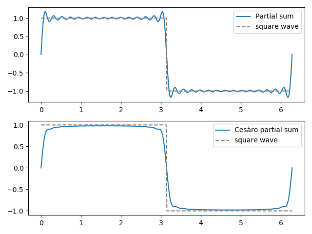
is Cesàro summation applied to Fourier series. The (ordinary) partial sums of a Fourier series give the best approximation to a function as measured by least squares norm. But the Cesàro partial sums may be qualitatively more like the function being approximated. We demonstrate this below with a square wave.

The 30th ordinary partial sum shows the beginnings of Gibbs phenomenon, the “bat ears” at the top of the square wave and their mirror image at the bottom. The 30th Cesàro partial sum is smoother and eliminates Gibbs phenomena near the discontinuity in the square wave.

More Fourier series posts

The worst tool for the job

I don’t recall where I read this, but someone recommended that if you need a tool, buy the cheapest one you can find. If it’s inadequate, or breaks, or you use it a lot, then buy the best one you can afford. (Update: Thanks to Jordi for reminding me in the comments that this comes from Kevin Kelly.)

If you follow this strategy, you’ll sometimes waste a little money by buying a cheap tool before buying a good one. But you won’t waste money buying expensive tools that you rarely use. And you won’t waste money by buying a sequence of incrementally better tools until you finally buy a good one.

The advice above was given in the context of tools you’d find in a hardware store, but I’ve been thinking about it in the context of software tools. There’s something to be said for having crude tools that are convenient for small tasks, and sophisticated tools that are appropriate for big tasks, but not investing much in the middle. That’s kind of what I was getting at in my recent post From shell to system.

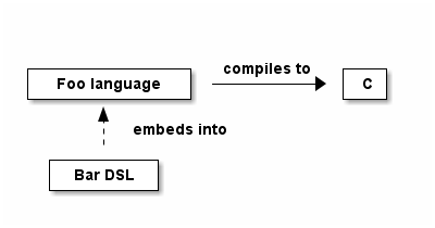
I’m making a bunch of diagrams for a new project, and the best tool for the job would probably be Adobe Illustrator because professionals routinely use it to make high-quality vector art. But I’m not doing that. I’m drawing ASCII art diagrams, just boxes and arrows drawn in plain text. Something like the drawing below.

  +--------------+ compiles to +---+  
  | Foo language | ----------> | C |  
  +--------------+             +---+  
         ^
         | embeds into
         :
    +---------+
    | Bar DSL |
    +---------+

The crude nature of ASCII art is a feature, not a bug. There is no temptation to be precious [*] about the aesthetics since the end product isn’t going to win any design awards in any case. There are compelling incentives to keep the diagrams small and simple. It encourages keeping the focus on content and give up on aesthetics once you hit diminishing return, which occurs fairly quickly.

Drawing ASCII diagrams is clumsy, even with tools that make it easier. Wouldn’t it be faster to use a tool meant for drawing? Well, yes and no. Drawing individual graphic elements would be faster in a drawing tool. But inevitably I’d spend more time on the appearance of the graphs, and so ultimately it would be slower.

The initial motivation for making ASCII diagrams was to keep diagrams and source code in the same file, not to eliminate the temptation to spend too much time tweaking graphics. The latter was a positive unintended consequence.

Related post: Doing good work with bad tools

***

I’m not doing this completely bare-knuckles. Emacs has tools like artist-mode that make it easier than manually positioning every character. And I’m using  DITAA sometimes to compile the plain text diagrams into graphics more appropriate for pasting into a report. The example above compiles to the image below.

DITAA example

More on how this works here.

***

[*] Not precious as in valuable, but precious as in affectedly or excessively refined. As in filmmaker Darren Doane’s slogan “We are not precious here.”

Not even close

Devil's Tower in Montana

Very often what cannot be done exactly can be done approximately. For example, most integrals cannot be computed in closed form, but they can be calculated numerically as closely as you’d like. But sometimes things are impossible, and you can’t even come close.

An impossible assignment

When I was in college, I had a friend who had a job in an engineering lab. The director of his lab had asked him to find an analytic analog to a smoothed indicator function. (I’ll say in more detail what that means shortly.) He mentioned the problem to me, and I told him there’s a theorem that says his assignment is impossible [1].

My friend was not deterred by my answer, confident that as an engineer he could find a practical way to do what mathematicians say can’t be done. That’s often a useful attitude, though not in this instance. Looking back, I can see how I could have given him a more useful reply than simply saying his task couldn’t be done; I could have explained why it cannot even be done approximately.

No exact plateaus

The indicator function of an interval is a function that takes on the value 1 on the interval and 0 everywhere else. This is a discontinuous function, but it can be approximated by a smooth function. Given a little transition zone on either end, you can have the function be zero on one side, one on the other, and ramp up smoothly in between. You can do this with infinitely differentiable functions, so why can’t you do something similar with analytic functions?

An analytic function can be expressed as a power series, and a power series is determined by its values in a small neighborhood of where it is centered. If you look at a patch where the function is zero, all its derivatives are zero, and so all the series coefficients are zero, and the function is zero. So the function’s value is zero everywhere. An analytic function can’t have a plateau without being flat everywhere.

No approximate plateaus

But can an analytic function have an approximate plateau? Can you construct an analytic function that is nearly 1 on some region, say a disk, and nearly 0 outside of some thin boundary around the disk [2]? In more picturesque language, can you construct an analytic function whose absolute value looks like Devil’s Tower in the photo above?

The barrier to creating something like Devil’s Tower is the maximum modulus principle. It says that the absolute value of an analytic function cannot have an interior maximum; the maximum always occurs on the boundary.

Suppose you’re trying to construct a function f(z) such that |f(z)| is a approximately zero within a radius 1 of the origin and approximately 0 outside a disk of radius 2. The first part is possible but the second part is not. The function f(z) cannot be perfectly flat on top without being constant everywhere (Liouville’s theorem) and the maximum of |f(z)| over the unit disk must occur somewhere on the rim of the disk (maximum modulus principle). However, it could be that f doesn’t vary much on the disk, and so there’s not much difference between its maximum and minimum over the disk.

Now consider the disk of radius 2. Somewhere on the rim, the circle of radius 2, |f(z)| must be larger than it was on the unit disk, or else |f(z)| would have an interior maximum, which the maximum modulus principle says cannot happen. |f(z)| might be small along parts of the circle of radius 2, but somewhere on that circle it is approximate 1 or larger.

Fake plateaus

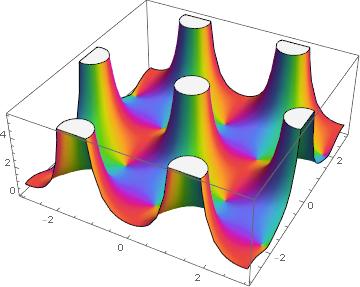
Sometimes you will see plots of analytic functions that do look flat on top, but that’s because singularities have been chopped off. Here’s such a plot from a blog post in a while back, a plot of Weierstrass’ elliptic function. The white plateaus are artifacts of cutting infinite values to fit in a finite box.


Complex plot of Weierstrass elliptic function

Related posts

[1] I wondered for a second how my friend’s supervisor couldn’t know this, then I realized it was probably a setup. His supervisor had given him an impossible task so that he’d struggle with it and learn why it was impossible.

[2] You could construct an analytic function that approximates a plateau along a one-dimensional slice, say along the real axis, but that approximation cannot be good in all directions.

Overview of NIST post-quantum encryption finalists

If and when large-scale quantum computing becomes practical, most public key encryption algorithms currently in use would be breakable. Cryptographers have known this since Peter Shor published his quantum factoring algorithm in 1994.

In 2017 researchers submitted 69 algorithms to the NIST Post-Quantum Cryptography Standardization Process. In 2019 NIST chose 26 of these algorithms to advance to the second round of competition. Yesterday NIST announced the finalists for the third round of its post-quantum cryptography competition.

The four finalists for public key encryption and key establishment management (KEM) are

  • Classic McEliece
  • CRYSTALS-KYBER
  • NTRU
  • SABER

The three finalists for digital signatures are

  • CRYSTALS-DILITHIUM
  • FALCON
  • Rainbow

There were five alternates for public key encryption/KEM

  • BIKE
  • FrodoKEM
  • HQC
  • NTRU Prime
  • SIKE

and three alternates for digital signatures

  • GeMSS
  • Picnic
  • SPHINCS+

Classic McEliece is a code-based encryption method. This terminology makes no sense if you think of codes and encryption as synonymous. Here “code” is being used in the sense of codes as in error-correcting codes.

Rainbow is an “unbalanced oil and vinegar” (UOV) algorithm. I wrote an introduction to UOV here.

The rest of the finalist algorithms (CRYSTALS-KYBER, NTRU, SABER, CRYSTALS-DILITHIUM, and FALCON) are all variations on the theme of learning with errors: RLWE (ring learning with errors), MLWE (module learning with errors), MLWR (module learning with rounding), etc. These are all based on the assumption that the analog of linear regression over a discrete ring or module is a hard problem, and would remain hard for quantum computers.

Among the alternates, SIKE is the only one involving elliptic curves. Shor’s algorithm makes it practical to solve the discrete logarithm problem for elliptic curves, and quantum computers could break traditional elliptic curve cryptography. But SIKE uses isogeny-based encryption. It doesn’t depend on the inner workings of individual elliptic curves but rather the isogenies between different elliptic curves.

The NIST report says that SIKE didn’t make the list of finalists because it was an order of magnitude slower than its competitors. But on the plus side, SIKE uses smaller keys and produces smaller cypher texts than the other methods. If researches find ways to speed up SIKE significantly, and if other researchers don’t find weaknesses in the method, it could be widely adopted in the future.

***

More posts on encryption.

Banned math book

Courant & Hilbert is a classic applied math textbook, still in print nearly a century after the first edition came out. The actual title of the book is Methods of Mathematical Physics, but everyone calls it Courant & Hilbert after the authors, Richard Courant and David Hilbert. I was surprised to find out recently that this was once a banned book. How could there be anything controversial about a math book? It doesn’t get into any controversial applications of math; it applies math to physics problems, but doesn’t apply the physics to anything in particular.

The book was first published in Germany in 1924 under the title Methoden der mathematischen Physik. Courant says in the preface

… I had been forced to leave Germany and was fortunate and grateful to be given the opportunities open in the United States. During the Second World War the German book became unavailable and was even suppressed by the National Socialist rulers of Germany. The survival of the book was secured when the United States Government seized the copyright and licensed a reprint issued by Interscience Publishers.

Courant’s language is remarkably restrained under the circumstances.

I wondered why the book was banned. Was Courant Jewish? I’d never considered this before, because I couldn’t care less about the ethnicity of authors. Jew or Greek, bond or free, male or female, I just care about their content. The Nazis, however, did care. According to his Wikipedia biography, Courant fled Germany not because of his Jewish ancestry but because of his affiliation with the wrong political party.

***

I never had Courant & Hilbert as a textbook, but I was familiar with it as a student. I vaguely remember that the library copy was in high demand and that I considered buying a copy, though it was too expensive for my means at the time. I recently bought a copy now that the book is cheaper and my means have improved.

I covered most of the material in Courant & Hilbert in graduate school, albeit in a more abstract form. As I mentioned the other day, my education was somewhat top-down; I learned about things first in an abstract setting and got down to particulars later, moving from soft analysis to hard analysis.

One quick anecdote along these lines. I read somewhere that David Hilbert was at a conference where someone referred to a Hilbert space and he asked the speaker what such a thing was. Hilbert’s work had motivated the definition of a Hilbert space, but Mr. Hilbert thought in more concrete terms.

Hadamard’s upper bound on determinant

For an n by n real matrix A, Hadamard’s upper bound on determinant is

 |A|^2 \leq \prod_{i=1}^n \sum_{j=1}^n a_{ij}^2

where aij is the element in row i and column j. See, for example, [1].

How tight is this upper bound? To find out, let’s write a little Python code to generate random matrices and compare their determinants to Hadamard’s bounds. We’ll take the square root of both sides of Hadamard’s inequality to get an upper bound on the absolute value of the determinant.

Hadamard’s inequality is homogeneous: multiplying the matrix A by λ multiplies both sides by λn. We’ll look at the ratio of Hadamard’s bound to the exact determinant. This has the same effect as generating matrices to have a fixed determinant value, such as 1.

    
    from scipy.stats import norm
    from scipy.linalg import det
    import matplotlib.pyplot as plt
    import numpy as np
    
    # Hadamard's upper bound on determinant squared
    def hadamard(A):
        return np.prod(np.sum(A**2, axis=1))
                
    N = 1000
    ratios = np.empty(N)
    
    dim = 3
    for i in range(N):
        A = norm.rvs(size=(dim, dim))
        ratios[i] = hadamard(A)**0.5/abs(det(A))
    
    plt.hist(ratios, bins=int(N**0.5))
    plt.show()
    

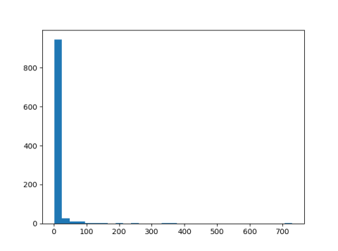
In this simulation the ratio is very often around 25 or less, but occasionally much larger, 730 in this example.

histogram

It makes sense that the ratio could be large; in theory the ratio could be infinite because the determinant could be zero. The error is frequently much smaller than the histogram might imply since a lot of small values are binned together.

I modified the code above to print quantiles and ran it again.

    print(min(ratios), max(ratios))
    qs = [0.05, 0.25, 0.5, 0.75, 0.95]
    print( [np.quantile(ratios, q) for q in qs] )

This printed

    1.0022 1624.9836
    [1.1558, 1.6450, 2.6048, 5.7189, 32.49279]

So while the maximum ratio was 1624, the ratio was less than 2.6048 half the time, and less than 5.7189 three quarters of the time.

Hadamard’s upper bound can be very inaccurate; there’s no limit on the relative error, though you could bound the absolute error in terms of the norm of the matrix. However, very often the relative error is moderately small.

More posts on determinants

[1] Courant and Hilbert, Methods of Mathematical Physics, Volume 1.

Cosine power approximation to normal

Ten years ago I wrote about how cosine makes a decent approximation to the normal (Gaussian) probability density. It turns out you get a much better approximation if you raise cosine to a power.

If we normalize cosk(t) by dividing by its integral

\int_{-\pi/2}^{\pi/2} \cos^k(t)\, dt = \sqrt{\pi}\,\, \frac{\Gamma\left( \frac{k+1}{2}\right) }{\Gamma\left( \frac{k+2}{2}\right)}

we get an approximation to the density function for a normal distribution with mean 0 and variance 1/k.

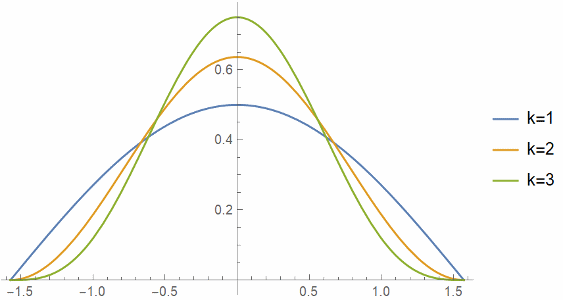
Here are the plots of cosk(t), normalized to integrate to 1, for k = 1, 2, and 3.

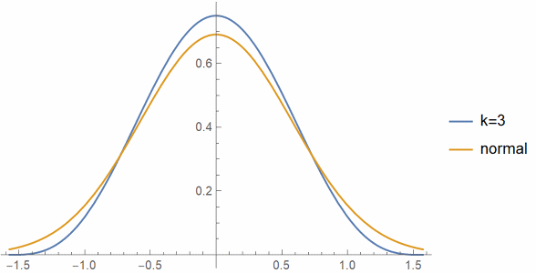
And here’s a plot of cos3(t) compared to a normal with variance 1/3.

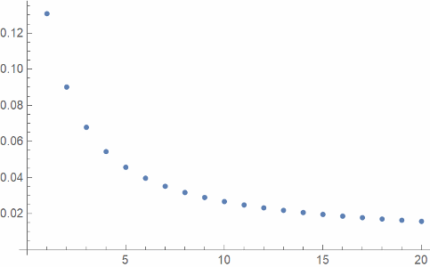
And finally here’s a plot of L² error, the square root of the integral of the square of the approximation error, as a function of k.

Update: You can do much better if you take a convex combination of cosine with 1 and allow non-integer powers. See this post.

Expressiveness

Programmers like highly expressive programming languages, but programming managers do not. I wrote about this on Twitter a few months ago.

Q: Why do people like Lisp so much?

A: Because Lisp is so expressive.

Q: Why don’t teams use Lisp much?

A: Because Lisp is so expressive.

Q: Why do programmers complain about Java?

A: Because it’s not that expressive.

Q: Why do businesses use Java?

A: Because it’s not that expressive.

A highly expressive programming language offers lots of options. This can be a good thing. It makes programming more fun, and it can lead to better code. But it can also lead to more idiosyncratic code.

A large programming language like Perl allows developers to carve out language subsets that hardly overlap. A team member has to learn not only the parts of the language he understands and wants to use, but also all the parts that his colleagues might use. And those parts that he might accidentally use.

While Perl has maximal syntax, Lisp has minimal syntax. But Lisp is also very expressive, albeit in a different way. Lisp makes it very easy to extend the language via macros. While Perl is a big language, Lisp is an extensible language. This can also lead to each programmer practically having their own language.

With great expressiveness comes great responsibility. A team using a highly expressive language needs to develop conventions for how the language will be used in order to avoid fracturing into multiple de facto languages.

But what if you’re a team of one? Now you don’t need to be as concerned how other people use your language. You still may need to care somewhat. You want to be able to grab sample code online, and you may want to share code or ask others for help. It pays not to be entirely idiosyncratic, though you’re free to wander further from the mainstream.

Even when you’re working in a team, you still may have code that only you use. If your team is producing C# code, and you secretively use a Perl script to help you find things in the code, no one needs to know. On the other hand, there’s a tendency for personal code to become production code, and so personal tools in a team environment are tricky.

But if you’re truly working by yourself, you have great freedom in your choice of tools. This can take a long time to sort out when you leave a team environment to strike out on your own. You may labor under your previous restrictions for a while before realizing they’re no longer necessary. At the same time, you may choose to stick to your old tools, not because they’re optimal for your new situation, but because it’s not worth the effort to retool.

Related posts

(Regarding the last link, think myth as in Joseph Campbell, not myth as in Myth Busters.)