The set of functions of the form
f(z) = (az + b)/(cz + d)
with ad ≠ bc are called bilinear transformations or Möbius transformations. These functions have three degrees of freedom—there are four parameters, but multiplying all parameters by a constant defines the same function—and so you can uniquely determine such a function by picking three points and specifying where they go.
Here’s an explicit formula for the Möbius transformation that takes z1, z2, and z3 to w1, w2, and w3.

To see that this is correct, or at least possible, note that if you set z = zi and w = wi for some i then two rows of the matrix are equal and so the determinant is zero.
Triangles, lines, and circles
You can pick three points in one complex plane, the z-plane, and three points in another complex plane, the w-plane, and find a Möbius transformation w = f(z) taking the z-plane to the w-plane sending the specified z‘s to the specified w‘s.
If you view the three points as vertices of a triangle, you’re specifying that one triangle gets mapped to another triangle. However, the sides of your triangle may or may not be straight lines.
Möbius transformations map circles and lines to circles and lines, but a circle might become a line or vice versa. So the straight lines of our original triangle may map to straight lines or they may become circular arcs. How can you tell whether the image of a side of a triangle will be straight or curved?
When does a line map to a line?
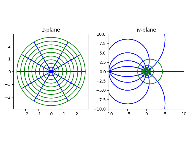
It’ll be easier if we add a point ∞ to the complex plane and think of lines as infinitely big circles, circles that pass through ∞.
The Möbius transformation (az + b)/(cz + d) takes ∞ to a/c and it takes −d/c to ∞.
The sides of a triangle are line segments. If we look at the entire line, not just the segment, then this line is mapped to a circle. If this line contains the point that gets mapped to ∞ then the image of the line is an infinite circle (i.e. a line). Otherwise the image of the line is a finite circle.
The line between z1 and z2 can be parameterized by
z1 + t(z2 − z1)
where t is real. So the image of this line will be a line if and only if
z1 + t(z2 − z1) = −d/c
for some real t. So solve for t and see whether you get a real number.
Note that if the point that is mapped to ∞ lies inside the line segment, not just on the line, then the image of that side of the triangle is infinitely long.
Examples
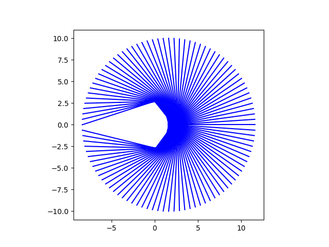
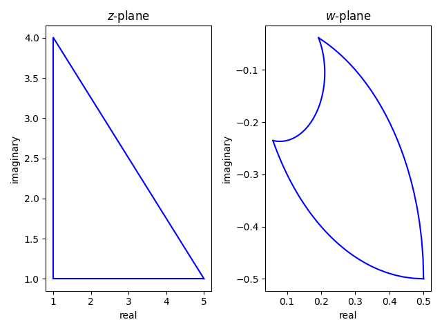
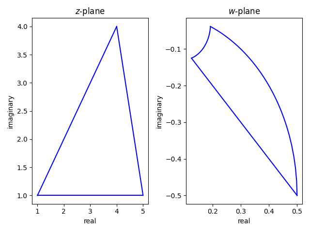
To keep things as simple as possible without being trivial, we’ll use the Möbius transformation f(z) = 1/z. Clearly the origin is the point that is mapped to ∞. The side of a triangle is mapped to a straight line if and only if the side is part of a line through the origin.
First let’s look at the triangle with vertices at (1, 1), (1, 4), and (5, 1). None of the sides is on a line that extends to the origin, so all sides map to circular arcs.
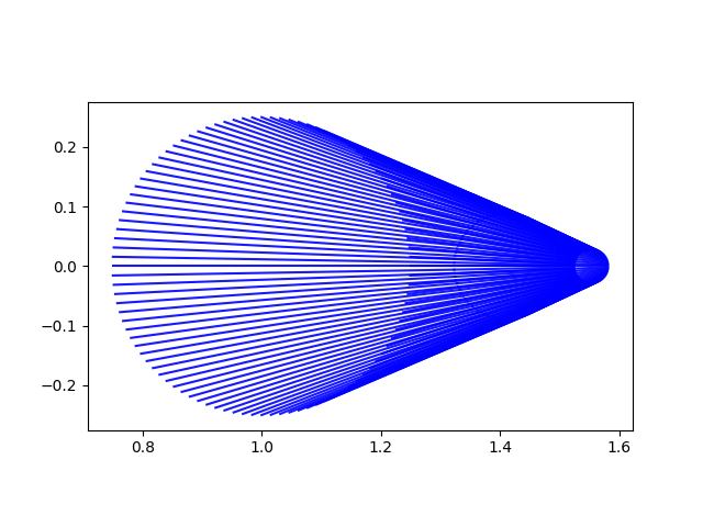
Next let’s move the second point from (1, 4) to (4, 4). The line running between (1, 1) and (4, 4) goes through the origin, and so the segment along that line maps to a straight line.
Related posts