Laplacian in various coordinate systems

Posted on 14 June 2021 by John

The recent post on the wave equation on a disk showed that the Laplace operator has a different form in polar coordinates than it does in Cartesian coordinates. In general, the Laplacian is not simply the sum of the second derivatives with respect to each variable.

Mathematica has a function, unsurprisingly called Laplacian, that will compute the Laplacian of a given function in a given coordinate system. If you give it a specific function, it will compute the Laplacian of that function. But you can also give it a general function to find a general formula.

For example,

    Simplify[Laplacian[f[r, θ], {r, θ}, "Polar"]]

returns

$\frac{f^{(0,2)}(r,\theta )}{r^2}+\frac{f^{(1,0)}(r,\theta )}{r}+f^{(2,0)}(r,\theta )$

This is not immediately recognizable as the Laplacian from this post

$\Delta u = \frac{\partial^2 u}{\partial r^2} + \frac{1}{r} \frac{\partial u}{\partial r} + \frac{1}{r^2} \frac{\partial^2 u}{\partial \theta^2}$

because Mathematica is using multi-index notation, which is a little cumbersome for simple cases, but much easier to use than classical notation when things get more complicated. The superscript (0,2), for example, means do not differentiate with respect to the first variable and differentiate twice with respect to the second variable. In other words, take the second derivative with respect to θ.

Here’s a more complicated example with oblate spheroidal coordinates. Such coordinates come in handy when you need to account for the fact that our planet is not exactly spherical but is more like an oblate spheroid.

When we ask Mathematica

    Simplify[Laplacian[f[ξ, η, φ], {ξ, η, φ}, "OblateSpheroidal"]]

the result isn’t pretty.

$(Csc[\[Eta]]^2*Sech[\[Xi]]^2*Derivative[0, 0, 2][f][\[Xi], \[Eta], \[Phi]] + (2*(Cot[\[Eta]]*Derivative[0, 1, 0][f][\[Xi], \[Eta], \[Phi]] + Derivative[0, 2, 0][f][\[Xi], \[Eta], \[Phi]] + Tanh[\[Xi]]*Derivative[1, 0, 0][f][\[Xi], \[Eta], \[Phi]] + Derivative[2, 0, 0][f][\[Xi], \[Eta], \[Phi]]))/ (Cos[2*\[Eta]] + Cosh[2*\[Xi]]))/\[FormalA]^2$

I tried using TeXForm and editing it into something readable, but after spending too much time on this I gave up and took a screenshot. But as ugly as the output is, it would be uglier (and error prone) to do by hand.

Mathematica supports the following 12 coordinate systems in addition to Cartesian coordinates:

Cylindrical
Bipolar cylindrical
Elliptic cylindrical
Parabolic cylindrical
Circular parabolic
Confocal paraboloidal
Spherical
Bispherical
Oblate spheroidal
Prolate spheroidal
Conical
Toroidal

These are all orthogonal, meaning that surfaces where one variable is held constant meet at right angles. Most curvilinear coordinate systems used in practice are orthogonal because this simplifies a lot of things.

Laplace’s equation is separable in Stäckel coordinate systems. These are all these coordinate systems except for toroidal coordinates. And in fact Stäckel coordinates are the only coordinate systems in which Laplace’s equation is separable.

It’s often the case that Laplace’s equation is separable in orthogonal coordinate systems, but not always. I don’t have a good explanation for why toroidal coordinates are an exception.

If you’d like a reference for this sort of thing, Wolfram Neutsch’s tome Coordinates is encyclopedic. However, it’s expensive new and hard to find used.

Lambert W strikes again

Posted on 23 April 2021 by John

I was studying a statistics paper the other day in which the author said to solve

t log( 1 + n/t ) = k

for t as part of an algorithm. Assume 0 < k < n.

Is this well posed?

First of all, can this equation be solved for t? Second, if there is a solution, is it unique?

It’s not hard to show that as a function of t, the left side approaches 0 as t approaches 0, and it approaches n as t goes to infinity. So there is a solution for all k between 0 and n. The restriction on k is necessary since the left side cannot exceed n.

With a little more work one can show that the derivative is always positive, so the left side is a monotonically increasing function, and so the solution given each value of k is unique.

Analytic solution

Now if we fix n, we can think of the equation above as defining t as a function of k. Can we solve for t exactly? I suspected that there might be a solution in terms of the Lambert W function because if you divide by t and exponentiate, you get an equation that smells like the equation

z = w exp(w)

defining the function W(z). It turns out this is indeed the case.

If we ask Mathematica

    Solve[t Log[1 + n/t] ==  k, t]

we get

$t\to -\frac{k}{ W\left(-\cfrac{k \exp(-k/n)}{n}\right)+\cfrac{k}{n}}$

Great! There’s a closed-form solution, if you accept using the W function as being closed form.

Problems with the solution

I found the solution in Mathematica, but I tested it in Python to make sure both platforms define W the same way.

    from numpy import log, exp
    from scipy.special import lambertw

    def f(t, n):
        return t*log(1 + n/t)

    def g(k, n):
        r = k/n
        return -k/(lambertw(-r*exp(-r)) + r)

    n, k = 10, 8
    t = g(k, n)
    print(f(t, n))

This should print k, so it prints 8, right? No, it prints 10.

What’s up with that?

If we look back at the equation for t above, we see that the W function is being evaluated at x exp(x) where x = –k/n, so we should get –k/n back since W(x exp(x)) = x by definition. But that means our denominator is zero, and so the equation doesn’t make sense!

Things are getting worse. At first we had a wrong value, but at least it was finite!

The problem is not a difference between Mathematica and Python.

Resolution

The problem is we’ve glossed over a branch cut of the W function. To make a long story short, we were using the principal branch of the W function, but we should have used a different branch.

Let’s go back to where I asked Mathematica

    Solve[t Log[1 + n/t] == k, t]

I ran the solution through TeXForm to get the TeX code that produced the image for the solution equation. I made a few aesthetic changes to the TeX, but it was essentially Mathematica’s output.

Without the TeXForm, Mathematica’s solution was in terms of ProductLog, not in terms of W; the TeXForm function turned ProductLog into W. If you look up ProductLog, it will tell you

ProductLog[z] gives the principal solution for w in z = we^w.

The principal solution. So we should be on the alert for difficulties with branches. There are two real solutions to z = we^w for some values of z, and we have to choose the right one. For example, if z = -0.1, the w could be -0.1118 or -3.5772.

Mathematica gave me the wrong branch. But to be fair, it did try to warn me.

Solve::ifun: Inverse functions are being used by Solve, so some solutions may not be found; use Reduce for complete solution information.

The solution is to use the -1 branch. In Mathematica’s notation, the branch comes before the argument. In SciPy, the branch comes second. So to fix the code above, we need to change

    lambertw(-r*exp(-r))

   lambertw(-r*exp(-r), -1)

and then the code will be correct.

If x is negative, and we use the -1 branch of W, then

W_-1(x exp(x)) ≠ x

and so we’re not dividing by zero in our solution.

Does chaos imply period 3?

Posted on 10 April 2021 by John

Sharkovskii’s theorem says that if a continuous map f from an interval I to itself has a point with period 3, then it has a point with period 5. And if it has a point with period 5, then it has points with order 7, etc. The theorem has a chain of implications that all begins with 3. If you have points with period 3, you have points of all periods.

Now suppose you want to go “upstream” in Sharkovskii’s chain of implications. If you have a point with period 5, do you have a point with period 3? The answer is no: a map can have points with period 5 without having points of period 3, though it necessarily has points with all other positive integer periods except 3.

There’s an example illustrating the claim above that I’ve seen in multiple places, but I haven’t seen it presented graphically. You could work through the example analytically, but here I present it graphically.

This is the example function written in Python.

    def f(x):
        assert(1 <= x <= 5)
    
        if x < 2:
            return 1 + 2*x
        if x < 3:
            return 7 - x
        if x < 4:
            return 10 - 2*x
        if x <= 5:
            return 6 - x

Here’s a graphical demonstration that f has a fixed point, but no points of period 3.

The only point fixed under applying f three times is the point that was already fixed under applying f once.

This graph shows that f has points with period 5:

By Sharkovskii’s theorem f must have points with all other periods, except 3. Here’s a demonstration that it has points with period 6.

The map f is chaotic, but it does not have a point with period 3.

Logistic map

Let’s look at the most famous chaotic map, the logistic map.

f(x) = rx (1 – x)

where x is in [0, 1] and r is in [0. 4].

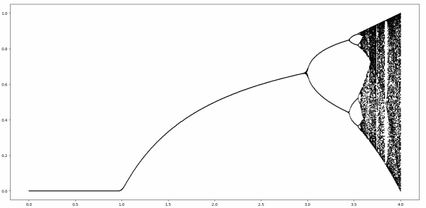
logistic bifurcation diagram

The images above shows orbits as r ranges over [0, 4]. Clearly f has points with period 2. There’s a whole interval of values of r that lead to points with period 2, roughly for r between 3 and 3.5. And we can see for r a little bigger there are points of period 4. But is there any point with period 3?

We can look for points of period 3 at the end of the plot, where r = 4, using Mathematica.

Define

    f[x_] := 4 x (1 - x)

and look for points where f³(x) = x using

    Factor[f[f[f[x]]] - x]

This shows that the solutions are the roots of

x (-3 + 4 x) (-7 + 56x – 112x² + 64 x³) (-3 + 36x – 96x² + 64x³)

The first two roots are fixed points, points of period 1, but the roots of the two cubic factors are points with period 3.

The cubics clearly have all their roots in the interval [0,1] and we could find their numerical values with

    NSolve[f[f[f[x]]] == x, x]

Although the roots are fixed points, they are unstable fixed points, as demonstrated at the bottom the next post.

Fourier uncertainty principle

Posted on 17 March 2021 by John

Heisenberg’s uncertainty principle says there is a limit to how well you can know both the position and momentum of anything at the same time. The product of the uncertainties in the two quantities has a lower bound.

There is a closely related principle in Fourier analysis that says a function and its Fourier transform cannot both be localized. The more concentrated a signal is in the time domain, the more spread out it is in the frequency domain.

There are many ways to quantify how localized or spread out a function is, and corresponding uncertainty theorems. This post will look at the form closest to the physical uncertainty principle of Heisenberg, measuring the uncertainty of a function in terms of its variance. The Fourier uncertainty principle gives a lower bound on the product of the variance of a function and the variance of its Fourier transform.

Variance

When you read “variance” above you might immediately thing of variance as in the variance of a random variable. Variance in Fourier analysis is related to variance in probability, but there’s a twist.

If f is a real-valued function of a real variable, its variance is defined to be

$V(f) = \int_{-\infty}^\infty x^2 \, f(x)^2 \, dx$

This is the variance of a random variable with mean 0 and probability density |f(x)|². The twist alluded to above is that f is not a probability density, but |f(x)|² is.

Since we said f is a real-valued function, we could leave out the absolute value signs and speak of f(x)² being a probability density. In quantum mechanics applications, however, f is complex-valued and |f(x)|² is a probability density. In other words, we multiply f by its complex conjugate, not by itself.

The Fourier variance defined above applies to any f for which the integral converges. It is not limited to the case of |f(x)|² being a probability density, i.e. when |f(x)|² integrates to 1.

Uncertainty principle

The Fourier uncertainty principle is the inequality

$V(f) \, \, V(\hat{f}) \geq C\, ||f||_2^2 \,\,||\hat{f}||_2^2$

where the constant C depends on your convention for defining the Fourier transform [1]. Here ||f||₂² is the integral of f², the square of the L² norm.

Perhaps a better way to write the inequality is

$\frac{V(f)}{||\phantom{\hat{f}}\!\!f\,||_2^2} \; \frac{V(\hat{f})}{||\phantom{\hat{.}}\hat{f}\,\,||_2^2} \geq C$

for non-zero f. Rather than look at the variances per se, we look at the variances relative to the size of f. This form is scale invariant: if we multiply f by a constant, the numerators and denominators are multiplied by that constant squared.

The inequality is exact when f is proportional to a Gaussian probability density. And in this case the uncertainty is easy to interpret. If f is proportional to the density of a normal distribution with standard deviation σ, then its Fourier transform is proportional to the density of a normal distribution with standard deviation 1/σ, if you use the radian convention described in [1].

Example

We will evaluate both sides of the Fourier uncertainty principle with

    h[x_] := 1/(x^4 + 1)

and its Fourier transform

    g[w_] := FourierTransform[h[x], x, w]

We compute the variances and the squared norms with

    v0 = Integrate[x^2 h[x]^2, {x, -Infinity, Infinity}] 
    v1 = Integrate[w^2 g[w]^2, {w, -Infinity, Infinity}]
    n0 = Integrate[    h[x]^2, {x, -Infinity, Infinity}]
    n1 = Integrate[    g[w]^2, {w, -Infinity, Infinity}]

The results in mathematical notation are

$\begin{align*} V(h) &= \frac{\pi}{4 \sqrt{2}} \\ V(\hat{h}) &= \frac{5\pi}{8\sqrt{2}} \\ || h ||_2^2 &= \frac{3\pi}{4 \sqrt{2}} \\ ||\hat{h}||_2^2 &= \frac{3\pi}{4 \sqrt{2}} \end{align*}$

From here we can calculate that the ratio of the left side to the right side of the uncertainty principle is 5/18, which is larger than the lower bound C = 1/4.

By the way, it’s not a coincidence that h and its Fourier transform have the same norm. That’s always the case. Or rather, that is always the case with the Fourier convention we are using here. In general, the L² norm of the Fourier transform is proportional to the L² norm of the function, where the proportionality constant depends on your definition of Fourier transform but not on the function.

Here is a page that lists the basic theorems of Fourier transforms under a variety of conventions.

[1] In the notation of the previous post C = 1/(4b²). That is, C = 1/4 if your definition has a term exp(± i ω t) and C = 1/16π² if your definition has a exp(±2 π i ω t) term.

Said another way, if you express frequency in radians, as is common in pure math, C = 1/4. But if you express frequency in Hertz, as is common in signal processing, C = 1/16π².

Fourier transform definitions also have varying constants outside the integral, e.g. possibly dividing by √2π, but this factor effects both sides of the Fourier uncertainty principle equally.

Fourier transforms in Mathematica

Posted on 17 March 2021 by John

Unfortunately there are many slightly different ways to define the Fourier transform. So the first two questions when using Mathematica (or any other software) to compute Fourier transforms are what definition of Fourier transform does it use, and what to do if you want to use a different definition.

The answer to the first question is that Mathematica defines the Fourier transform of f as

$\hat{f}(\omega) = \frac{1}{\sqrt{2\pi}} \int_{-\infty}^\infty \exp(i\omega x)\, f(x) \, dx$

The answer to the second question is that Mathematica defines a parameterized Fourier transform by

$\hat{f}(\omega) = \sqrt{\frac{|b|}{(2\pi)^{1-a}}} \, \int_{-\infty}^\infty \exp(ib\omega x)\, f(x) \, dx$

where a defaults to 0 and b defaults to 1.

Examples

For example, if φ(x) = exp(-x²/2), then we can compute Mathematica’s default Fourier transform with

    φ[x_] := Exp[-x^2/2]
    FourierTransform[φ[x], x, ω]

This computes

$\hat{\varphi}(\omega) = \frac{1}{\sqrt{2\pi}} \int_{-\infty}^\infty \exp(i\omega x)\, \varphi(x) \, dx = \exp(-\omega^2/2)$

But if we set (a, b) to (0, 2π) with

    FourierTransform[φ[x], x, ω, FourierParameters -> {0, 2 Pi}]

we compute

$\hat{\varphi}(\omega) = \int_{-\infty}^\infty \exp(2\pi i\omega x)\, \varphi(x) \, dx = \sqrt{2\pi} \exp(-2\pi^2\omega^2/2)$

Theorems under various conventions

Several years ago I got frustrated enough with the multitude of Fourier transform conventions that I made a sort of Rosetta Stone, giving several of the most basic theorems under each of eight definitions. I used the parameterization

$\hat{f}(\omega) = \frac{1}{\sqrt{m}} \int_{-\infty}^\infty \exp(\sigma q i\omega x)\, f(x) \, dx$

where m is either 1 or 2π, σ is either 1 or -1, and q is either 1 or 2π.

My σ and q are the sign and absolute value of Mathematica’s b. The relation between my m and Mathematica’s a is slightly more complicated and given in the table below.

$\begin{tabular}{lllll} \hline $\sigma$ & m & q & a & b\\ \hline \textpm{} 1 & 1 & 1 & 1 & \textpm{} 1\\ \textpm{} 1 & 1 & 2$\pi$ & 0 & \textpm{} 2$\pi$\\ \textpm{} 1 & 2$\pi$ & 1 & 0 & \textpm{} 1\\ \textpm{} 1 & 2$\pi$ & 2$\pi$ & -1 & \textpm{} 2$\pi$\\ \hline \end{tabular}$

Adding tubes to knots

Posted on 7 March 2021 by John

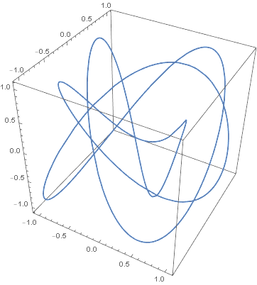
Several months ago I wrote a blog post about Lissajous curves and knots that included the image below.

Lissajous knot

Here’s an improved version of the same knot.

Lissajous knot plotted in Mathematica with Tube function

The original image was like tying the knot in thread. The new image is like tying it in rope, which makes it easier to see. The key was to use Mathematica’s Tube function to thicken the curve and to see the crossings. I also removed the bounding box in the image.

This was the original code:

    x[t_] := Cos[3 t]
    y[t_] := Cos[4 t + Sqrt[2]]
    z[t_] := Cos[5 t + Sqrt[3]]
   
    ParametricPlot3D[{x[t], y[t], z[t]}, {t, 0, 2 Pi}]

The new code keeps the definitions of x, y, and z but creates a plot using Tube.

    
    Graphics3D[
        Tube[
             Table[{x[i], y[i], z[i]}, {i, 0, 2 Pi, 0.01}], 
             0.05
        ], 
        Boxed -> False
    ]

I went back and changed out the plots in my post Total curvature of a knot with plots similar to the one above.

Pythagorean dates

Posted on 16 December 2020 by John

The numbers that make up today’s date—12, 16, and 20—form a Pythagorean triple. That is, 12² + 16² = 20².

There won’t be any such dates next year. You could confirm this by brute force since there are only 365 days in 2021, but I hope to do something a little more interesting here.

The Mathematica function

    PowersRepresentations[n, k, p]

lists the ways to represent a number n as the sum of k pth powers. Calling PowersRepresentations[21^2, 2, 2] shows that there is no non-trivial way to write 21² as the sum of two powers; the only way is 0² + 21². You might try using the whole year rather than the last two digits, but there’s no non-trivial way to write 2021 as the sum of two powers either.

The paragraph above says that no Pythagorean triangle can have hypotenuse 21 or 2021. But could there be a Pythagorean date next year with 21 on one of the sides?

If the components of a date correspond to sides of a Pythagorean triangle, and one of the sides is 21, then the day must be on the hypotenuse because all the month numbers are less than 21, and that day must be greater than 21.

Let’s look for Pythagorean triangles with a side equal to 22, 23, …, 31 and see whether any of them have a 21 on the side.

The Mathematica command

    For[d = 22, d <= 31, d++, Print[PowersRepresentations[d*d, 2, 2]]]

returns

    {{0,22}}
    {{0,23}}
    {{0,24}}
    {{0,25},{7,24},{15,20}}
    {{0,26},{10,24}}
    {{0,27}}
    {{0,28}}
    {{0,29},{20,21}}
    {{0,30},{18,24}}
    {{0,31}}

This tells us that the only numbers from 22 to 31 that can be on the side of a Pythagorean triangle are 25, 26, 29, and 30.

The number 21 does appear in the list: (20, 21, 29) is a Pythagorean triple. But if the 29th of a month were a Pythagorean date next year, it would have to be the 20th month. Since we only have 12 months, there won’t be any Pythagorean dates next year.

The number 22, 23, and 24 can’t be written as sums of squares in a non-trivial way, so if there’s a Pythagorean date in the next few years it will have to be with the day of the month on the side. We can see from the output above that (7, 24, 25) is a Pythagorean triple, so the next Pythagorean date is 7/25/24, and the next after that is 7/24/25. And the next after that will be 10/24/26.

Incidentally, there is an algorithm for counting how many ways a number can be written as the sum of k squares, and it is implemented in Mathematica as Squares[k, n]. If you run SquaresR[2, 441] it will tell you that there are four ways to write 441 as the sum of two squares. But all four of these are trivial: (0, 21), (21, 0), (0, -21), and (-21, 0). Because every square can be written as the sum of two squares analogously, a return value of 4 means there are no non-trivial solutions.

New Asymptotic function in Mathematica 12.1

Posted on 20 March 2020 by John

One of the new features in Mathematica 12.1 is the function Asymptotic. Here’s a quick example of using it.

Here’s an asymptotic series for the log of the gamma function I wrote about here.

$\log \Gamma(z) \sim (z - \frac{1}{2}) \log z - z + \frac{1}{2} \log(2\pi) + \frac{1}{12z} - \frac{1}{360z^3} + \cdots$

If we ask Mathematica

    Asymptotic[LogGamma[z], z -> Infinity]

we get simply the first term:

But we can set the argument SeriesTermGoal to tell it we’d like more terms. For example

    Asymptotic[LogGamma[z], z -> Infinity, SeriesTermGoal -> 4]

yields

This doesn’t contain a term 1/z⁴, but it doesn’t need to: there is no such term in the asymptotic expansion, so it is giving us the terms up to order 4, it’s just that the coefficient of the 1/z⁴ term is zero.

If we ask for terms up to order 5

    Asymptotic[LogGamma[z], z -> Infinity, SeriesTermGoal -> 5]

we do get a term 1/z⁵, but notice there is no 4th order term.

A note on output forms

The Mathematica output displayed above was created by using

Export[filename, expression]

to save images as SVG files. The alt text for the images was created using

InputForm[expression].

Chebyshev approximation

Posted on 11 March 2020 by John

In the previous post I mentioned that Remez algorithm computes the best polynomial approximation to a given function f as measured by the maximum norm. That is, for a given n, it finds the polynomial p of order n that minimizes the absolute error

|| f – p ||_∞.

The Mathematica function MiniMaxApproximation minimizes the relative error by minimizing

|| (f – p) / f ||_∞.

As was pointed out in the comments to the previous post, Chebyshev approximation produces a nearly optimal approximation, coming close to minimizing the absolute error. The Chebyshev approximation can be computed more easily and the results are easier to understand.

To form a Chebyshev approximation, we expand a function in a series of Chebyshev polynomials, analogous to expanding a function in a Fourier series, and keep the first few terms. Like sines and cosines, Chebyshev polynomials are orthogonal functions, and so Chebyshev series are analogous to Fourier series. (If you find it puzzling to hear of functions being orthogonal to each other, see this post.)

Here is Mathematica code to find and plot the Chebyshev approximation to e^x over [-1, 1]. First, here are the coefficients.

    weight[x_] := 2/(Pi Sqrt[1 - x^2])
    c = Table[ 
        Integrate[ Exp[x] ChebyshevT[n, x] weight[x], {x, -1, 1}], 
        {n, 0, 5}]

The coefficients turn out to be exactly expressible in terms of Bessel functions, but typically you’d need to do a numerical integration with NIntegrate.

Now we use the Chebyshev coefficients to evaluate the Chebyshev approximation.

    p[x_] := Evaluate[c . Table[ChebyshevT[n - 1, x], {n, Length[c]}]] 
             - First[c]/2

You could see the approximating polynomial with

    Simplify[N[p[x]]]

which displays

    1.00004 + 1.00002 x + 0.499197 x^2 + 0.166489 x^3 + 0.0437939 x^4 + 
 0.00868682 x^5

The code

    Plot[Exp[x] - p[x], {x, -1, 1}]

shows the error in approximating the exponential function with the polynomial above.

Note that the plot has nearly equal ripples; the optimal approximation would have exactly equal ripples. The Chebyshev approximation is not optimal, but it is close. The absolute error is smaller than that of MiniMaxApproximation by a factor of about e.

There are bounds on how different the error can be between the best polynomial approximation and the Chebyshev series approximation. For polynomials of degree n, the Chebyshev error is never more than

4 + 4 log(n + 1)/π

times the optimal approximation error. See Theorem 16.1 in Approximation Theory and Approximation Practice by Lloyd N. Trefethen.

Remez algorithm and best polynomial approximation

Posted on 10 March 2020 by John

The best polynomial approximation, in the sense of minimizing the maximum error, can be found by the Remez algorithm. I expected Mathematica to have a function implementing this algorithm, but apparently it does not have one. (But see update below.)

It has a function named MiniMaxApproximation which sounds like Remez algorithm, and it’s close, but it’s not it.

To use this function you first have to load the FunctionApproximations package.

    << FunctionApproximations`

Then we can use it, for example, to find a polynomial approximation to e^x on the interval [-1, 1].

    MiniMaxApproximation[Exp[x], {x, {-1, 1}, 5, 0}]

This returns the polynomial

    1.00003 + 0.999837 x + 0.499342 x^2 + 0.167274 x^3 + 0.0436463 x^4 + 
 0.00804051 x^5

And if we plot the error, the difference between e^x and this polynomial, we see that we get a good fit.

minimax error

But we know this isn’t optimal because there is a theorem that says the optimal approximation has equal ripple error. That is, the absolute value of the error at all its extrema should be the same. In the graph above, the error is quite a bit larger on the right end than on the left end.

Still, the error is not much larger than the smallest possible using 5th degree polynomials. And the error is about 10x smaller than using a Taylor series approximation.

    Plot[Exp[x] - (1 + x + x^2/2 + x^3/6 + x^4/24 + x^5/120), {x, -1, 1}]

minimax error

Update: Jason Merrill pointed out in a comment what I was missing. Turns out MiniMaxApproximation finds an approximation that minimizes relative error. Since e^x doesn’t change that much over [-1, 1], the absolute error and relative error aren’t radically different. There is no option to minimize absolute error.

When you look at the approximation error divided by e^x you get the ripples you’d expect.

minimax error

See the next post for a way to construct near optimal polynomial approximations using Chebyshev approximation.

Mathematica

Laplacian in various coordinate systems

Lambert W strikes again

Is this well posed?

Analytic solution

Problems with the solution

Resolution

More posts with Lambert W

Does chaos imply period 3?

Logistic map

Related posts

Fourier uncertainty principle

Variance

Uncertainty principle

Example

Related posts

Fourier transforms in Mathematica

Examples

Theorems under various conventions

Adding tubes to knots

Pythagorean dates

New Asymptotic function in Mathematica 12.1

A note on output forms

More Mathematica posts

Chebyshev approximation

More Chebyshev posts

Remez algorithm and best polynomial approximation