Jacobi functions are complex-valued functions of a complex variable z and a parameter m. Often this parameter is real, and 0 ≤ m < 1. Mathematical software libraries, like Python’s SciPy, often have this restriction. However, m could be any complex number.
The previous couple of posts spoke of the fundamental rectangle for Jacobi functions. But in general, Jacobi functions (and all other elliptic functions) have a fundamental parallelogram.
When m is real, the two periods of the Jacobi sn function are 4K(m) and 2K(1-m) i and so the function repeats horizontally and vertically. (Here K is the complete elliptic integral of the first kind.) When m is complex, the two periods are again 4K(m) and 2K(1-m) i, but now 4K(m) and 2K(1-m) are complex numbers and their ratio is not necessarily real. This means sn repeats over a parallelogram which is not necessarily a rectangle.
The rest of the post will illustrate this with plots.
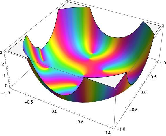
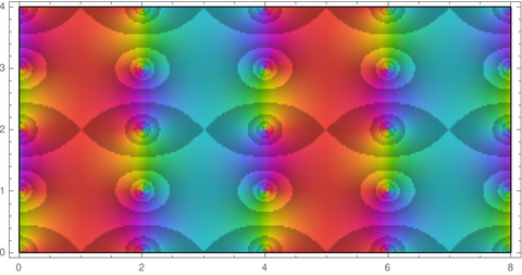
First, here is a plot of sn(K(1/2)z, 1/2). The height of the graph represents the absolute value of the function and the color represents its phase. (The argument z was multiplied by K(1/2) to make the periods have integer values, making it a little easier to see the periods.)
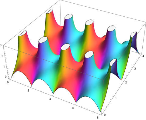
Notice that the plot features line up with the coordinate axes, the real axis running from 0 to 8 in the image and the complex axis running from 0 to 4.
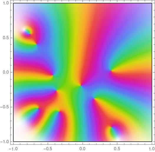
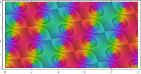
Here’s the analogous plot for sn(z, 2 + 2i).
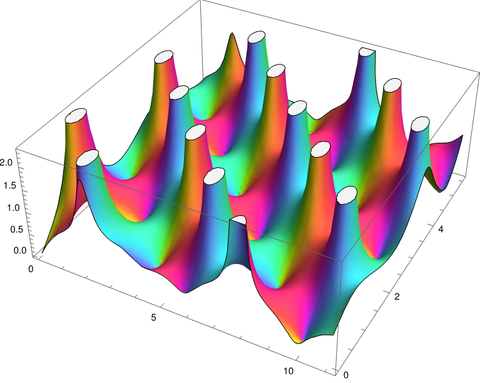
Now the features are running on a diagonal. The pits are where the function is zero and the white ellipses are poles that have the tops cut off to fit in a finite plot.
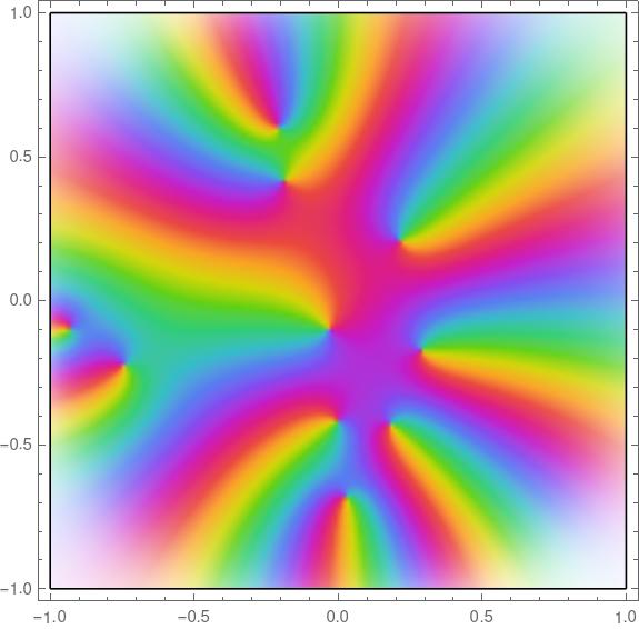
It will be easier to see what’s going on if we switch to flat plots. The color represents phase as before, but now magnitude is denoted by contour lines.
Here’s a plot of sn(K(1/2)z, 1/2)
and here’s a plot of sn(z, 2 + 2i).
According to theory the two periods should be
4 K(2 + 2i) = 4.59117 + 2.89266 i
and
2i K(-1 – 2i) = -1.44633 + 2.29559 i.
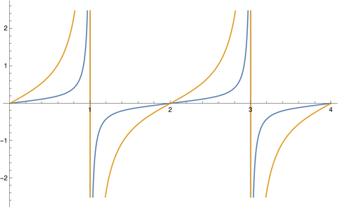
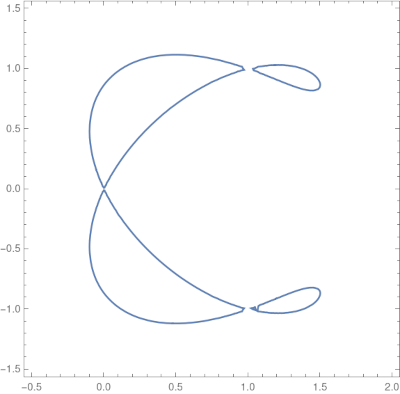
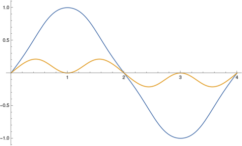
We can show that this is the case by plotting the real and imaginary parts of sn(z, 2 + 2i) as we move in these two directions.
The Mathematica code
    Plot[
        {Re[JacobiSN[t EllipticK[2 + 2 I], (2 + 2 I)]],
         Im[JacobiSN[t EllipticK[2 + 2 I], (2 + 2 I)]]},
        {t, 0, 4}]
produces this plot
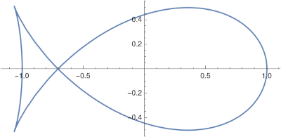
and the code
    Plot[
        {Re[JacobiSN[t I EllipticK[-1 - 2 I], (2 + 2 I)]],
         Im[JacobiSN[t I EllipticK[-1 - 2 I], (2 + 2 I)]]},
        {t, 0, 4}]
produces this plot.