Analogies between Weierstrass functions and trig functions

If you look at the Wikipedia article on Weierstrass functions, you’ll find a line that says “the relation between the sigma, zeta, and ℘ functions is analogous to that between the sine, cotangent, and squared cosecant functions.” This post unpacks that sentence.

Weierstrass p function

First of all, what is ℘? It’s the Weierstrass elliptic function, which is the mother of all elliptic functions in some sense. All other elliptic functions can be constructed from this function and its derivatives. As for the symbol itself, ℘ is the traditional symbol for the Weierstrass function. It’s U+2118 in Unicode, ℘ in HTML, and \wp in LaTeX.

The line above suggests that ℘(x) is analogous to csc²(x). Indeed, the plots of the two functions are nearly identical.

Here’s Weierstrass’ function:

Weierstrass p plot

And here’s csc²:

plot of csc^2

The two plots basically agree to within the thickness of a line.

The Weierstrass function ℘ has two parameters that I haven’t mentioned. Elliptic functions are periodic in two directions in the complex plane, and so their values everywhere are determined by their values over a parallelogram. The two parameters specify the fundamental parallelogram, or at least that’s one way of parametrizing the function. The WeierstrassP function in Mathematica takes two other parameters, called the invariants, and these invariants were chosen in the plot above to match the period of the cosecant function.

    Plot[Sin[x]^-2, {x, -10, 10}]
    Plot[WeierstrassP[
            x, 
            WeierstrassInvariants[{Pi/2, Pi I/2}]
         ], 
        {x, -10, 10}
    ]

The fundamental parallelogram is defined in terms of half periods, usually denoted with ω’s, and the invariants are denoted with g‘s. The function WeierstrassInvariants converts from half periods to invariants, from ω’s to g‘s.

Note that ℘ and cosecant squared are similar along the real axis, but they’re very different in the full complex plane. Trig functions are periodic along the real axis but grow exponentially along the complex axis. Elliptic functions are periodic along both axes.

Weierstrass zeta function

The Weierstrass zeta function is not an elliptic function. It is not periodic but rather quasiperiodic. The derivative of the Weierstrass zeta function is negative of the Weierstrass elliptic function, i.e.

ζ ‘(x) = -℘(x)

which is analogous to the fact that the derivative of cot(x) is -csc²(x). So in that sense ζ is to ℘ as cotangent is to cosecant squared.

The plots of ζ(x) and cot(x) are similar as shown below.

Plot of Weierstrass zeta and cotangent

The Mathematica code to make the plot above was

    Plot[
        {WeierstrassZeta[x, WeierstrassInvariants[{Pi/2, Pi I/2}]], 
         Cot[x]}, 
        {x, -10, 10}, 
        PlotLabels -> {"zeta", "cot"}
    ]

Weierstrass sigma function

The Weierstrass sigma function is also not an elliptic function. It is analogous to the sine function as follows. The logarithmic derivative of the Weierstrass sigma function is the Weierstrass zeta function, just as the logarithmic derivative of sine is cotangent. That is,

(log(σ(x))’ = ζ(x).

The logarithmic derivative of a function is the derivative of its log, and so the logarithmic derivative of a function f is f ‘ / f.

However, the plot of the sigma function, WeierstrassSigma in Mathematica, hardly looks line sine.

Plot of Weierstrass sigma and sine

So in summary, logarithmic derivative takes Weierstrass sigma to Weierstrass zeta just as it takes sine to cotangent. Negative derivative takes Weierstrass zeta to Weierstrass ℘ just as it takes cotangent to negative cosecant squared.

Related elliptic function posts

Total curvature of a knot

Tie a knot in a rope and join the ends together. At each point in the rope, compute the curvature, i.e. how much the rope bends, and integrate this over the length of the rope. The Fary-Milnor theorem says the result must be greater than 4π. This post will illustrate this theorem by computing numerically integrating the curvature of a knot.

If p and q are relatively prime integers, then the following equations parameterize a knot.

x(t) = cos(pt) (cos(qt) + 2)
y(t) = sin(pt) (cos(qt) + 2)
z(t) = -sin(qt)

This is in fact a torus knot because the curve stays on the surface of a torus (doughnut) [1]. We can get a trefoil knot, for example, by setting p = 2 and q = 3.

Trefoil knot

We’ll use Mathematica to compute the total curvature of this knot and other examples. First the parameterization:

    x[t_, p_, q_] := Cos[p t] (Cos[q t] + 2)
    y[t_, p_, q_] := Sin[p t] (Cos[q t] + 2) 
    z[t_, p_, q_] := -Sin[q t]

We can plot torus knots as follows.

    k[t_, p_, q_] := { 
        x[t, p, q], 
        y[t, p, q], 
        z[t, p, q]
    }
    Graphics3D[Tube[Table[k[i, p, q], {i, 0, 2 Pi, 0.01}], 
        0.08], Boxed -> False]

Here’s a more complicated knot with p = 3 and q = 7.

(3, 7) knot

Before we can integrate the curvature with respect to arc length, we need an expression for an element of arc length as a function of the parameter t.

    ds[t_, p_, q_] :=  Sqrt[ 
        D[x[t, p, q], t]^2 + 
        D[y[t, p, q], t]^2 + 
        D[z[t, p, q], t]^2
    ]

Now we can compute the total curvature.

    total[p_, q_] := NIntegrate[
        ArcCurvature[k[t, p, q], t] ds[t, p, q], 
        {t, 0, 2 Pi}
    ]

We can use this to find that the total curvature of the (2,3) torus knot, the trefoil, is 17.8224, whereas 4π is 12.5664. So the Fary-Milnor theorem holds.

Let’s do one more example, this time a (1,4) knot.

unknot

You can see that this is not actually knot. This doesn’t contradict what we said above because 1 divides 4. When p or q equal 1, we get an unknot.

When we compute its total curvature we get 24.2737, more than 4π. The Fary-Milnor theorem doesn’t say that total curvature in excess of 4π is a sufficient condition for a loop to be knotted; it says it’s necessary. Total curvature less than 4π proves that something isn’t a knot, but curvature greater than 4π doesn’t prove anything.

More on curvature and knots

[1] If you change out the 2s in the parameterization with a larger number, it’s easier to see from the graphs that the curves are on a torus. For example, if we plot the (3,7) knot again, replacing 2’s in the definition of x(t) and y(t) with 5’s, we can kinda see a torus inside the knot.

(3, 7) knot torus

Uniform approximation paradox

What I’m going to present here is not exactly a paradox, but I couldn’t think of a better way to describe it in the space of a title. I’ll discuss two theorems about uniform convergence that seem to contradict each other, then show by an example why there’s no contradiction.

Weierstrass approximation theorem

One of my favorite theorems is the Weierstrass approximation theorem. It says that every continuous function can be approximated as closely as you like by polynomials. This is surprising because polynomials are very special, well behaved functions, and merely continuous function can be worse.

For example, a polynomial cannot have any kinks in it, unlike the absolute value function. But even though an individual polynomial cannot have a kink, a sequence of polynomials can approach a kink.

Morera’s theorem

Morera’s theorem [1] says that the uniform limit of analytic functions is analytic. But Weierstrass’s theorem says that the uniform limit of analytic functions (namely polynomials) can have a kink in it, which an analytic function cannot have. What gives?

Weierstrass’s theorem is about uniform convergence over an interval of the real line.

Morera’s theorem is about uniform convergence on compact subsets of an open set in the complex plane.

We’ll show an example below where a sequence of polynomials converges to |x| on an interval of the real line but not in a disk containing the interval.

Bernstein polynomials

The Weierstrass approximation theorem tells us that there exists a sequence of polynomials converging uniformly to any continuous function on a compact interval. But we can go a step further and actually construct a sequence of such polynomials. The polynomials fall out of a proof of the Weierstrass theorem using probability! There’s nothing random going on here, and yet we can take a set of inequalities that fall out of calculations motivated by probability and construct our approximations.

Here is the nth Bernstein polynomial approximation to a function g in Mathematica code.

B[x_, n_, g_] := 
    Sum[Binomial[n, k] x^k (1 - x)^(n - k) g[k/n], 
        {k, 0, n}]

We can then use the following code to show the convergence of Bernstein polynomials.

f[x_] := Abs[x - 1/2]
Plot[{B[x, 4, f], B[x, 10, f], B[x, 30, f], f[x]}, 
    {x, 0, 1} , PlotLegends -> "Expressions"]

Plot of Bernstein polynomials converging to absolute value

Next we’ll take a particular Bernstein polynomial for f in the sequence and plot the difference between it and f over the complex plane.

ComplexPlot3D[B[z, 6, f] - f[z], {z, 0, 1 + I}]

Bernstein approximation error in complex plane

The polynomial is close to f along the interval [0, 1] on the real line, but the further we move away from the real axis the further it gets from f. Furthermore, the distance increases as we increase the degree of polynomial. The following code looks at the distance between Bn(i) and f(i) for n = 1, 2, 3, …, 10.

Table[N[Abs[B[I , n, f] - f[I]]], {n, 1, 10}]

It returns

 0.6180
 1.9021
 1.9021
 3.4085
 3.4085
 7.3941
 7.3941
23.4511
23.4511
92.4377

So there’s no contradiction between the theorems of Weierstrass and Morera. The Bernstein polynomials do indeed converge uniformly to f over [0, 1] but they do not converge in the complex plane.

More analysis posts

[1] I don’t know whether this theorem is exactly due to Morera, but it follows directly from Morera’s theorem.

Software to factor integers

In my previous post, I showed how changing one bit of a semiprime (i.e. the product of two primes) creates an integer that can be factored much faster. I started writing that post using Python with SymPy, but moved to Mathematica because factoring took too long.

SymPy vs Mathematica

When I’m working in Python, SymPy lets me stay in Python. I’ll often use SymPy for a task that Mathematica could do better just so I can stay in one environment. But sometimes efficiency is a problem.

SymPy is written in pure Python, for better and for worse. When it comes to factoring large integers, it’s for worse. I tried factoring a 140-bit integer with SymPy, and killed the process after over an hour. Mathematica factored the same integer in 1/3 of a second.

Mathematica vs PARI/GP

The previous post factors 200-bit semiprimes. The first example, N = pq where

p = 1078376712338123201911958185123
q = 1126171711601272883728179081277

took 99.94 seconds to factor using Mathematica. A random sample of 13 products of 100-bit primes and they took an average of 99.1 seconds to factor.

Using PARI/GP, factoring the value of N above took 11.4 seconds to factor. I then generated a sample of 10 products of 100-bit primes and on average they took 10.4 seconds to factor using PARI/GP.

So in these examples, Mathematica is several orders of magnitude faster than SymPy, and PARI/GP is one order of magnitude faster than Mathematica.

It could be that the PARI/GP algorithms are relatively better at factoring semiprimes. To compare the efficiency of PARI/GP and Mathematica on non-semiprimes, I repeated the exercise in the previous post, flipping each bit of N one at a time and factoring.

This took 240.3 seconds with PARI/GP. The same code in Mathematica took 994.5 seconds. So in this example, PARI/GP is about 4 times faster where as for semiprimes it was 10 times faster.

Python and PARI

There is a Python interface to PARI called cypari2. It should offer the convenience of working in Python with the efficiency of PARI. Unfortunately, the installation failed on my computer. I think SageMath interfaces Python to PARI but I haven’t tried it.

More on prime factoring

Calling Python from Mathematica

The Mathematica function ExternalEvalute lets you call Python from Mathematica. However, there are a few wrinkles.

I first pasted in an example from the Mathematica documentation and it failed.

    ExternalEvaluate[
        "Python", 
        {"def f(x): return x**2", "f(3)"}
    ]

It turns out you (may) have to tell Mathematica where to find Python. I ran the following, tried again, and the example worked.

    RegisterExternalEvaluator[
        "Python", 
        "C:\\bin\\Anaconda3\\python.EXE"
    ]

You can also run Python with NumPy loaded using

    ExternalEvaluate["Python-NumPy", … ]

except that didn’t work the first time either. You have to register a Python-NumPy evaluator separately. So I ran

    RegisterExternalEvaluator[
        "Python-NumPy", 
        "C:\\bin\\Anaconda3\\python.EXE"
    ]

and then tried again calling Python code using NumPy. But then there’s the question of how it imports NumPy. Does it simply run import numpy, or maybe from numpy import *, or maybe import numpy as np? It turns out the first possibility is what happens. So to print pi from NumPy, your code string needs to be numpy.pi.

You don’t need to use Python-NumPy if you just do your own importing. For example, this code returns π².

    ExternalEvaluate[
        "Python", 
        "import numpy; x = numpy.pi; x**2"
    ]

And you can import any library you’d like, not just NumPy.

    ExternalEvaluate[
        "Python", 
        "from sympy import isprime; isprime(7)"
    ]

Everything above applies to Mathematica 11.3 and Mathematica 12.

Higher dimensional squircles

The previous post looked at what exponent makes the area of a squircle midway between the area of a square and circle of the same radius. We could ask the analogous question in three dimensions, or in any dimension.

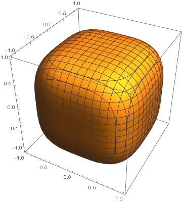
(What do you call a shape between a cube and a sphere? A cuere? A sphube?)


The sphube

In more conventional mathematical terminology, higher dimensional squircles are balls under Lp norms. The unit ball in n dimensions under the Lp norm has volume

2^n \frac{\Gamma\left(1 + \frac{1}{p}\right)^n}{\Gamma\left( 1 + \frac{n}{p} \right)}

We’re asking to solve for p so the volume of a p-norm ball is midway between that of 2-norm ball and an ∞-norm ball. We can compute this with the following Mathematica code.

    v[p_, n_] := 2^n Gamma[1 + 1/p]^n / Gamma[1 + n/p]
    Table[ 
        FindRoot[
            v[p, n] - (2^n + v[2, n])/2, 
            {p, 3}
        ], 
        {n, 2, 10}
    ]

This shows that the value of p increases steadily with dimension:

    3.16204
    3.43184
    3.81881
    4.33311
    4.96873
    5.70408
    6.51057
    7.36177
    8.23809

We saw the value 3.16204 in the previous post. The result for three dimensions is 3.43184, etc. The image above uses the solution for n = 3, and so it has volume halfway between that of a sphere and a cube.

In order to keep the total volume midway between that of a cube and a sphere, p has to increase with dimension, making each 2-D cross section more and more like a square.

Here’s the Mathematica code to draw the cuere/sphube.

    p = 3.43184
    ContourPlot3D[
         Abs[x]^p + Abs[y]^p + Abs[z]^p == 1, 
         {x, -1, 1}, 
         {y, -1, 1}, 
         {z, -1, 1}
    ]

Sine of a googol

How do you evaluate the sine of a large number in floating point arithmetic? What does the result even mean?

Sine of a trillion

Let’s start by finding the sine of a trillion (1012) using floating point arithmetic. There are a couple ways to think about this. The floating point number t = 1.0e12 can only be represented to 15 or 16 significant decimal figures (to be precise, 53 bits [1]), and so you could think of it as a representative of the interval of numbers that all have the same floating point representation. Any result that is the sine of a number in that interval should be considered correct.

Another way to look at this is to say that t can be represented exactly—its binary representation requires 42 bits and we have 53 bits of significand precision available—and so we expect sin(t) to return the sine of exactly one trillion, correct to full precision.

It turns out that IEEE arithmetic does the latter, computing sin(1e12) correctly to 16 digits.

Here’s the result in Python

    >>> sin(1.0e12)
    -0.6112387023768895

and verified by Mathematica by computing the value to 20 decimal places

    In:= N[Sin[10^12], 20]
    Out= -0.61123870237688949819

Range reduction

Note that the result above is not what you’d get if you were first to take the remainder when dividing by 2π and then taking the sine.

    >>> sin(1.0e12 % (2*pi))
    -0.6112078499756778

This makes sense. The result of dividing a trillion by the floating point representation of 2π, 159154943091.89536, is correct to full floating point precision. But most of that precision is in the integer part. The fractional part is only has five digits of precision, and so we should expect the result above to be correct to at most five digits. In fact it’s accurate to four digits.

When your processor computes sin(1e12) it does not naively take the remainder by 2π and then compute the sine. If it did, you’d get four significant figures rather than 16.

We started out by saying that there were two ways of looking at the problem, and according to the first one, returning only four significant figures would be quite reasonable. If we think of the value t as a measured quantity, measured to the precision of floating point arithmetic (though hardly anything can be measured that accurately), then four significant figures would be all we should expect. But the people who designed the sine function implementation on your processor did more than they might be expected to do, finding the sine of a trillion to full precision. They do this using a range reduction algorithm that retains far more precision than naively doing a division. (I worked on this problem a long time ago.)

Sine of a googol?

What if we try to take the sine of a ridiculously large number like a googol (10100)? This won’t work because a googol cannot be represented exactly as a floating point number (i.e. as a IEEE 754 double). It’s not too big; floating point numbers can be as large as around 10308. The problem is that a number that big cannot be represented to full precision. But we can represent 2333 exactly, and a googol is between 2332 and 2333. And amazingly, Python’s sine function (or rather the sine function built into the AMD processor on my computer) returns the correct result to full precision.

    >>> sin(2**333)
    0.9731320373846353

How do we know this is right? I verified it in Mathematica:

    In:= Sin[2.0^333]
    Out= 0.9731320373846353

How do we know Mathematica is right? We can do naive range reduction using extended precision, say 200 decimal places.

    In:= p = N[Pi, 200]
    In:= theta = x - IntegerPart[x/ (2 p)] 2 p
    Out= 1.8031286178334699559384196689…

and verify that the sine of the range reduced value is correct.

    In:= Sin[theta]
    Out= 0.97313203738463526…

Interval arithmetic interpretation

Because floating point numbers have 53 bits of precision, all real numbers between 256 – 22 and 256 + 22 are represented as the floating point number 256. This is a range of width 8, wider than 2π, and so the sines of the numbers in this range cover the possible values of sine, i.e. [-1, 1]. So if you think of a floating point number as a sample from the set of all real numbers with the same binary representation, every possible value of sine is a valid return value for numbers bigger than 256. But if you think of a floating point number as representing itself exactly, then it makes sense to ask for the sine of numbers like 2333 and larger, up to the limits of floating point representation [2].

More numerical math posts

[1] An IEEE 754 double has 52 significand bits, but these bits can represent 53 bits of precision because the first bit of the fractional part is always 1, and so it does not need to be represented. See more here.

[2] The largest exponent of an IEEE double is 1023, and the largest significand is 2 – 2-53 (i.e. all 1’s), so the largest possible value of a double is

(253 – 1)21024-53

and in fact the Python expression sin((2**53 - 1)*2**(1024-53)) returns the correct value to 16 significant figures.

Spherical trig, Research Triangle, and Mathematica

This post will look at the triangle behind North Carolina’s Research Triangle using Mathematica’s geographic functions.

Spherical triangles

A spherical triangle is a triangle drawn on the surface of a sphere. It has three vertices, given by points on the sphere, and three sides. The sides of the triangle are portions of great circles running between two vertices. A great circle is a circle of maximum radius, a circle with the same center as the sphere.

An interesting aspect of spherical geometry is that both the sides and angles of a spherical triangle are angles. Because the sides of a spherical triangle are arcs, they have angular measure, the angle formed by connecting each vertex to the center of the sphere. The arc length of a side is its angular measure times the radius of the sphere.

Denote the three vertices by AB, and C. Denote the side opposite A by a, etc. Denote the angles at AB, and C by α, β, and γ respectively.

Research Triangle

Research Triangle is a (spherical!) triangle with vertices formed by Duke University, North Carolina State University, and University of North Carolina at Chapel Hill.

(That was the origin of the name, though it’s now applied more loosely to the general area around these three universities.)

We’ll take as our vertices

  • A = UNC Chapel Hill (35.9046 N, 79.0468 W)
  • B = Duke University in Durham (36.0011 N, 78.9389 W),
  • C = NCSU in Raleigh (35.7872 N, 78.6705 W)

Research Triangle

Mathematica

We’ll illustrate several features of Mathematica using the spherical triangle corresponding to Research Triangle.

Map

The map above was produced with the following Mathematica code.

    ptA = GeoPosition[{35.9046, -79.0468}]
    ptB = GeoPosition[{36.0011, -78.9389}]
    ptC = GeoPosition[{35.7872, -78.6705}]

    GeoGraphics[{Red, PointSize[Large], 
        Point[ptA], Point[ptB], Point[ptC]}, 
        GeoScaleBar -> "Imperial", 
        GeoRange -> 29000]

Note that longitude is in degrees east, so the longitudes above are negative.

Distance

To find the distance between two locations, you can use the function GeoDistance. For example,

    GeoDistance[ptA, ptB]

tells me that the distance between UNC and Duke is 8.99185 miles. I assume it displays miles by default based on my location in the US, though the GeoRange option above defaults to meters. You can make the system of units explicit. For example

    GeoDistance[ptA, ptB, UnitSystem -> "Metric"]

returns 14.741 km.

If we want to find the length of the side c in degrees, we can use the Earth’s radius.

    r = PlanetData["Earth", "Radius"]
    c = GeoDistance[ptA, ptB] 360 / (2 Pi r)

This shows that c is 0.13014°. Calculating the other sides similarly shows a = 0.30504° and b = 0.32739°.

Angles

Calling GeoDirection[ptA, ptB] returns 42.2432°, which says we need to head at an angle of about 42° to walk from UNC to Duke.

The code

    GeoDirection[ptA, ptB] - GeoDirection[ptA, ptC]

shows that the angle α is 68.6128°. (The code returns the negative of this angle because the angle is clockwise.) Similarly we find β = 87.9808° and γ = 23.4068.

The angles add up to 180° only because our triangle is small compared to the earth’s total area. The actual sum should be slightly more than 180°, but we’ve not retained enough precision to detect the difference. In general the “spherical excess,” i.e. the amount by which the sum of the angles exceed 180°, is proportional to the area of the triangle.

More spherical trig posts

Prime denominators and nines complement

Let p be a prime. If the repeating decimal for the fraction a/p has even period, the second half of the decimals are the 9’s complement of the first half. This is known as Midy’s theorem.

For a small example, take

1/7 = 0.142857142857…

and notice that 142 + 857 = 999. That is, 8, 5, and 7 are the nine’s complements of 1, 4, and 2 respectively.

For a larger example, we can use Mathematica to look at the decimal expansion of 6/47:

    In:  N[6/47, 60]
    Out: 0.127659574468085106382978723404255319148936170212765957446809

and we can confirm

    12765957446808510638297 + 
    87234042553191489361702 =
    99999999999999999999999

Let’s do another example with 6/43:

    In:  N[6/43, 50]
    Out: 0.13953488372093023255813953488372093023255813953488

Does the theorem hold here? The the hypothesis of the theorem doesn’t hold because the fraction has period 21, which is not even. Can the conclusion of the theorem hold anyway? No, because we can’t split 21 digits in half! But we can split 21 digits into three parts, and if we do we find

    1395348 + 8372093 + 232558 = 9999999

Let’s finish up with an example in another base. We’ll look at the fraction 3/7 in base 17.

    In:  BaseForm[N[3/7, 24], 17]
    Out: 0.74e9c274e9c274e9c2717

If we split the repeating part of the decimal into two parts we get 74e and 9c2, and these add up to the base 17 analog of all 9’s.

    In:  BaseForm[17^^74e + 17^^9c2, 17]
    Out: ggg17

That is, the base 17 numbers 9, c, and 2, are the g’s complements of 7, 4, and e respectively.

[The Mathematica operator ^^ interprets its right argument as a number whose base is given by the left argument. The BaseForm function takes a number as its first argument and returns its representation in the base given as its second argument.]

Related post: Casting out Z’s

Continued fraction cryptography

Every rational number can be expanded into a continued fraction with positive integer coefficients. And the process can be reversed: given a sequence of positive integers, you can make them the coefficients in a continued fraction and reduce it to a simple fraction.

In 1954, Arthur Porges published a one-page article pointing out that continued fractions could be used to create a cipher. To encrypt your cleartext, convert it to a list of integers, use them as continued fraction coefficients, and report the resulting fraction. To decrypt, expand the fraction into a continued fraction and convert the coefficients back to text.

We can implement this in Mathematica as follows:

    
encode[text_] := FromContinuedFraction[ ToCharacterCode[ text ]]
decode[frac_] := FromCharacterCode[ ContinuedFraction[ frac ]]

So, for example, suppose we want to encrypt “adobe.” If we convert each letter to its ASCII code we get {97, 100, 111, 98, 101}. When we make these numbers coefficients in a continued fraction we get

\mathrm{

which reduces to 10661292093 / 109898899.

This isn’t a secure encryption scheme by any means, but it’s a cute one. It’s more of an encoding scheme, a (non-secret) way to convert a string of numbers into a pair of numbers.

Related posts

[1] Arthur Porges. A Continued Fraction Cipher. The American Mathematical Monthly, Vol. 59, No. 4 (Apr., 1952), p. 236