Logarithmic spiral

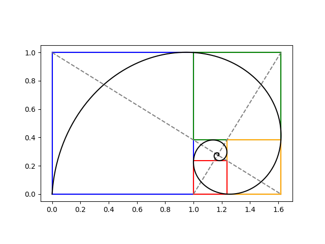
I’ve seen an image similar to the following many times, but I don’t recall any source going into detail regarding how the spiral is constructed. This post will do just that.

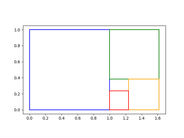
The previous post constructed iterated golden rectangles. We start with a golden rectangle and imagine chopping of first the blue, then the green, then the orange, and then the red square. We could continue this process on the inner most rectangle, over and over.

At this point, many sources would say “Hey look! We can draw a spiral that goes through two corners of each square” without explicitly stating an equation for the spiral. We’ll find spiral, making everything explicit.

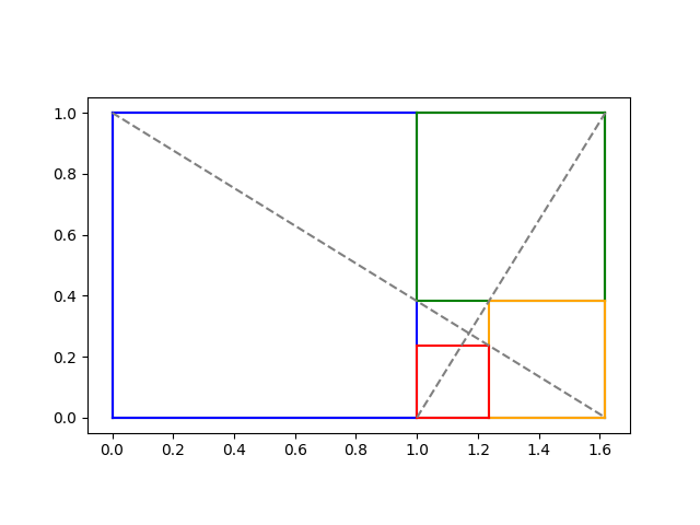
In the previous post we showed how to find the limit of the iterative process at the intersection of the two diagonal lines below.

We showed that the intersection is at

x0 = (2φ + 1)/(φ + 2)

and

y0 = 1/(φ + 2).

Logarithmic spirals

A logarithmic spiral centered at the origin has the polar equation

r(θ) = a exp(kθ)

for some constants a and k. Our spiral will be such a spiral shifted to center at (x0y0).

Imagine a spiral going from the lower left to the top left of the blue square, then to the top left of the green square, then to the top right of the orange square etc., passing through two corners of every square. Every time θ goes through a quarter turn, i.e. π/2 radians, our rectangles get smaller by a factor of φ. We can use this to solve for k because

a exp(k(θ + π/2)) = φ a exp()

and so

exp(kπ/2) = φ

and

k = 2log(φ) / π.

To summarize what we know so far, if we shift our spiral to the origin, it has equation in polar form

r(θ) = a exp(kθ)

where we now know k but don’t yet know a.

Finding θ and a

To get our actual spiral, we have to shift the origin to (x0, y0) which we have calculated above. Converting from polar to rectangular coordinates so we can do the shift, we have

x(θ) = x0 + a exp(kθ) cos(θ)

y(θ) = y0 + a exp(kθ) sin(θ)

We can find the parameter a by knowing that our spiral passes through the origin, the bottom left corner in the plots above. At what value of θ does the curve go through the origin? We have a choice; values of θ that differ by multiples of 2π will give different values of a.

The angle θ is the angle made by the line connecting (0, 0) to (x0, y0). We can find θ via

θ0 = atan2(−y0, −x0).

Here’s Python code to find θ0:

    import numpy as np

    phi = (1 + 5**0.5)/2
    y0 = 1/(2+phi)
    x0 = (2*phi + 1)*y0
    theta0 = np.arctan2(-y0, -x0)

Then we solve for a from the equation x0) = 0.

    k = 2*np.log(phi)/np.pi
    a = -x0 / (np.exp(k*theta0)*np.cos(theta0)))

Plots

Now we have all the parameters we need to define our logarithmic spiral. The following code draws our logarithmic spiral on top of the plot of the rectangles.

    t = np.linspace(-20, theta0, 1000)
    def x(t): return x0 + a*np.exp(k*t)*np.cos(t)
    def y(t): return y0 + a*np.exp(k*t)*np.sin(t)
    plt.plot(x(t), y(t), "k-")

The result is the image at the top of the post.

Non-associative multiplication

There are five ways to parenthesize a product of four things:

  • ((ab)c)d
  • (ab)(cd)
  • (a(b(cd))
  • (a(bc))d
  • (a((bc)d)

In a context where multiplication is not associative, the five products above are not necessarily the same. Maybe all five are different.

This post will give two examples where the products above are all different: octonions and matrix multiplication.

If you’re thinking “But wait: matrix multiplication is associative!” then read further and see in what sense I’m saying it’s not.

Octonions

Octonion multiplication is not associative. I wrote a blog post a while back asking how close the octonions come to being associative. That is, if we randomly generate unit-length octonions a, b, and c, we can calculate the norm of

(ab)ca(bc)

and ask about its expected value. Sometimes for a triple of octonions this value is zero, but on average this expression has norm greater than 1. I estimated the average value via simulation, and later Greg Egan worked out the exact value. His write-up had gone down with the Google+ ship, but recently Greg posted a new version of his notes.

In this post I gave Python code for multiplying octonions using a function called CayleyDickson named after the originators of the algorithm. Let’s rename it m to have something shorter to work with and compute all five ways of associating a product of four octonions.

    import numpy as np

    def m(x, y):
        return CayleyDickson(x, y)

    def take_five(a, b, c, d):
        return [
            m(a, (m(b, m(c, d)))),
            m(m(a, b), m(c, d)),
            m(m(m(a, b), c), d),
            m(a, m(m(b, c), d)),
            m(m(a, m(b, c)), d)
    ]

I first tried products of basis elements, and I only got two different products out of the five ways of associating multiplication, but I only tried a few examples. However, when I tried using four random octonions, I got five different products.

    np.random.seed(20220201)

    a = np.random.rand(8)
    b = np.random.rand(8)
    c = np.random.rand(8)
    d = np.random.rand(8)

    for t in take_five(a, b, c, d):
        print(t)

This gave a very interesting result: I got five different results, but only two different real (first) components. The five vectors all differed in the last seven components, but only produced two distinct first components.

    [ 2.5180856  -2.61618184  ...]
    [ 2.5180856   0.32031027  ...]
    [ 2.5180856   1.13177500  ...]
    [ 3.0280984  -0.30169446  ...]
    [ 3.0280984  -2.36523580  ...]

I repeated this experiment a few times, and the first three results always had the same real component, and the last two results had another real component.

I suspect there’s a theorem that says

Re( ((ab)c)d ) = Re( (ab)(cd) ) = Re( a(b(cd)) )

and

Re( (a(bc))d ) = Re( a((bc)d) )

but I haven’t tried to prove it. If you come with a proof, or a counterexample, please post a link in the comments.

Matrix multiplication

Matrix multiplication is indeed associative, but the efficiency of matrix multiplication is not. That is, any two ways of parenthesizing a matrix product will give the same final matrix, but the cost of the various products are not the same. I first wrote about this here.

This is a very important result in practice. Changing the parentheses in a matrix product can make the difference between a computation being practical or impractical. This comes up, for example, in automatic differentiation and in backpropagation for neural networks.

Suppose A is an m by n matrix and B is an n by p matrix. Then AB is an m by p matrix, and forming the product AB requires mnp scalar multiplications. If C is a by q matrix, then (AB)C takes

mnp + mpq = mp(n + q)

scalar multiplications, but computing A(BC) takes

npqmnq = nq(m + p)

scalar multiplications, and in general these are not equal.

Let’s rewrite our multiplication function m and our take_five function to compute the cost of multiplying four matrices of random size.

We’ve got an interesting programming problem in that our multiplication function needs to do two different things. First of all, we need to know the size of the resulting matrix. But we also want to keep track of the number of scalar multiplications the product would require. We have a sort of main channel and a side channel. Having our multiplication function return both the dimension and the cost would make composition awkward.

This is kind of a fork in the road. There are two ways to solving this problem, one high-status and one low-status. The high-status approach would be to use a monad. The low-status approach would be to use a global variable. I’m going to take the low road and use a global variable. What’s one little global variable among friends?

    mults = 0

    def M(x, y):
        global mults
        mults += x[0]*x[1]*y[0]
        return (x[0], y[1])

    def take_five2(a, b, c, d):

        global mults
        costs = []

        mults = 0; M(a, (M(b, M(c, d)))); costs.append(mults)
        mults = 0; M(M(a, b), M(c, d));   costs.append(mults)
        mults = 0; M(M(M(a, b), c), d);   costs.append(mults)
        mults = 0; M(a, M(M(b, c), d));   costs.append(mults)
        mults = 0; M(M(a, M(b, c)), d);   costs.append(mults)

        return costs 

Next, I’ll generate five random integers, and group them in pairs as sizes of matrices conformable for multiplication.

    dims = np.random.random_integers(10, size=5)
    dim_pairs = zip(dims[:4], dims[1:])
    c = take_five2(*[p for p in dim_pairs])

When I ran this dims was set to

[3 9 7 10 6]

and so my matrices were of size 3×9, 9×7, 7×10, and 10×6.

The number of scalar multiplications required by each way of multiplying the four matrices, computed by take_five2 was

[1384, 1090, 690, 1584, 984]

So each took a different number of operations. The slowest approach would take more than twice as long as the fastest approach. In applications, matrices can be very long and skinny, or very wide and thin, in which case one approach may take orders of magnitude more operations than another.

Related posts

Planetary code golf

Suppose you’re asked to write a function that takes a number and returns a planet. We’ll number the planets in order from the sun, starting at 1, and for our purposes Pluto is the 9th planet.

Here’s an obvious solution:

    def planet(n):
        planets = [
            "Mercury",
            "Venus",
            "Earth",
            "Mars",
            "Jupiter",
            "Saturn",
            "Uranus",
            "Neptune",
            "Pluto"
        ]
        # subtract 1 to correct for unit offset
        return planets[n-1] 

Now let’s have some fun with this and play a little code golf. Here’s a much shorter program.

    def planet(n): return chr(0x263e+n)

I was deliberately ambiguous at the top of the post, saying the code should return a planet. The first function naturally interprets that to mean the name of a planet, but the second function takes it to mean the symbol of a planet.

The symbol for Mercury has Unicode value U+263F, and Unicode lists the symbols for the planets in order from the sun. So the Unicode character for the nth planet is the character for Mercury plus n. That would be true if we numbered the planets starting from 0, but conventionally we call Mercury the 1st planet, not the 0th planet, so we have to subtract one. That’s why the code contains 0x263e rather than 0x263f.

We could make the function just a tiny bit shorter by using a lambda expression and using a decimal number for 0x263e.

    planet = lambda n: chr(9790+n)

Display issues

Here’s a brief way to list the symbols from the Python REPL.

    >>> [chr(0x263f+n) for n in range(9)]
    ['☿', '♀', '♁', '♂', '♃', '♄', '♅', '♆', '♇']

You may see the symbols for Venus and Mars above rendered with a colored background, depending on your browser and OS.

Here’s what the lines above looked like at my command line.

screen shot of repl

Here’s what the symbols looked like when I posted them on Twitter.

symbols for planets

For reasons explained here, some software interprets some characters as emoji rather than literal characters. The symbols for Venus and Mars are used as emoji for female and male respectively, based on the use of the symbols in biology. Incidentally, these symbols were used to represent planets long before biologists used them to represent sexes.

Related posts

Spaceship operator in Python

Some programming languages, such as Perl, have an infix operator <=> that returns a three-state comparison. The expression

    a <=> b

evaluates to -1, 0, or 1 depending on whether a < b, a = b, or a > b. You could think of <=> as a concatenation of <, =, and >.

The <=> operator is often called the “spaceship operator” because it looks like Darth Vader’s ship in Star Wars.

Python doesn’t have a spaceship operator, but you can get the same effect with numpy.sign(a-b). For example, suppose you wanted to write a program to compare two integers.

You could write

    from numpy import sign
    def compare(x, y):
        cmp = ["equal to", "greater than", "less than"][sign(x-y)]
        print(f"{x} is {cmp} {y}.")

Here we take advantage of the fact that an index of -1 points to the last element of a list.

The sign function will return an integer if its argument is an integer or a float if its argument is a float. The code above will break if you pass in floating point numbers because sign will return −1.0, 0.0, or 1.0. But if you replace sign(x-y) with int(sign(x-y)) it will work for floating point arguments.

Related post: Symbol pronunciation

Fraction comparison trick

If you want to determine whether

a/b > c/d,

it is often enough to test whether

a + d > b + c.

Said another way a/b is usually greater than c/d when a + d is greater than b + c.

This sounds imprecise if not crazy. But it is easy to make precise and [1] shows that it is true.

Examples

Consider 4/11 vs 3/7. In this case 4 + 7 = 11 < 11 + 3 = 14, which suggests 4/11 < 3/7, which is correct.

But the rule of thumb can lead you astray. For example, suppose you want to compare 3/7 and 2/5. We have 3 + 5 = 8 < 7 + 2 = 9, but 3/7 > 2/5.

The claim isn’t that the rule always works; clearly it doesn’t. The claim is that it usually works, in a sense that will be made precise in the next section.

Rigorous statement

Let N be a large integer, and pick integers a, b, c, and d at random uniformly between 1 and N. Let

x = a/bc/d

and

y = (a+d) − (b+c).

Then the probability x and y are both positive, or both negative, or both zero, approaches 11/12 as N goes to infinity.

Simulation

I won’t repeat the proof of the theorem above; see [1] for that. But I’ll give a simulation that illustrates the theorem.

    import numpy as np
    
    np.random.seed(20210225)
    
    N = 1_000_000
    numreps = 10_000
    
    count = 0
    for _ in range(numreps):
        (a, b, c, d) = np.random.randint(1, N+1, 4, dtype=np.int64)
        x = a*d - b*c
        y = (a+d) - (b+c)
        if np.sign(x) == np.sign(y):
            count += 1
    print(count/numreps)

This prints 0.9176, and 11/12 = 0.91666….

The random number generator randint defaults to 32-bit integers, but this could lead to overflow since 106 × 106 > 232. So I used 64-bit integers.

Instead of computing a/bc/d, I multiply by bd and compute adbc instead because this avoids any possible floating point issues.

In case you’re not familiar with the sign function, it returns 1 for positive numbers, 0 for 0, and −1 for negative numbers.

The code suggests a different statement of the theorem: if you generate two pairs of integers, their sums and their products are probably ordered the same way.

Psychology

This post has assumed that the numbers a, b, c, and d are all chosen uniformly at random. But the components of the fractions for which you have any doubt whether a/b is greater or less than c/d are not uniformly distributed. For example, consider 17/81 versus 64/38. Clearly the former is less than 1 and the latter is greater than 1.

It would be interesting to try to assess how often the rule of thumb presented here is correct in practice. You might try to come up with a model for the kinds of fractions people can’t compare instantly, such as proper fractions that have similar size.

Related posts

[1] Kenzi Odani. A Rough-and-Ready Rule for Fractions. The Mathematical Gazette, Vol. 82, No. 493 (Mar., 1998), pp. 107-109

Python triple quote strings and regular expressions

There are several ways to quote strings in Python. Triple quotes let strings span multiple lines. Line breaks in your source file become line break characters in your string. A triple-quoted string in Python acts something like “here doc” in other languages.

However, Python’s indentation rules complicate matters because the indentation becomes part of the quoted string. For example, suppose you have the following code outside of a function.

x = """\
abc
def
ghi
"""

Then you move this into a function foo and change its name to y.

def foo():
    y = """\
    abc
    def
    ghi
    """

Now x and y are different strings! The former begins with a and the latter begins with four spaces. (The backslash after the opening triple quote prevents the following newline from being part of the quoted string. Otherwise x and y would begin with a newline.) The string y also has four spaces in front of def and four spaces in front of ghi. You can’t push the string contents to the left margin because that would violate Python’s formatting rules. (Update: Oh yes you can! See Aaron Meurer’s comment below.)

We now give three solutions to this problem.

Solution 1: textwrap.dedent

There is a function in the Python standard library that will strip the unwanted space out of the string y.

import textwrap 

def foo():
    y = """\
    abc
    def
    ghi
    """
    y = textwrap.dedent(y)

This works, but in my opinion a better approach is to use regular expressions [1].

Solution 2: Regular expression with a flag

We want to remove white space, and the regular expression for a white space character is \s. We want to remove one or more white spaces so we add a + on the end. But in general we don’t want to remove all white space, just white space at the beginning of a line, so we stick ^ on the front to say we want to match white space at the beginning of a line.

import re 

def foo():
    y = """\
    abc
    def
    ghi
    """
    y = re.sub("^\s+", "", y)

Unfortunately this doesn’t work. By default ^ only matches the beginning of a string, not the beginning of a line. So it will only remove the white space in front of the first line; there will still be white space in front of the following lines.

One solution is to add the flag re.MULTILINE to the substitution function. This will signal that we want ^ to match the beginning of every line in our multi-line string.

    y = re.sub("^\s+", "", y, re.MULTILINE)

Unfortunately that doesn’t quite work either! The fourth positional argument to re.sub is a count of how many substitutions to make. It defaults to 0, which actually means infinity, i.e. replace all occurrences. You could set count to 1 to replace only the first occurrence, for example. If we’re not going to specify count we have to set flags by name rather than by position, i.e. the line above should be

    y = re.sub("^\s+", "", y, flags=re.MULTILINE)

That works.

You could also abbreviate re.MULTILINE to re.M. The former is more explicit and the latter is more compact. To each his own. There’s more than one way to do it. [2]

Solution 3: Regular expression with a modifier

In my opinion, it is better to modify the regular expression itself than to pass in a flag. The modifier (?m) specifies that in the rest of the regular the ^ character should match the beginning of each line.

    y = re.sub("(?m)^\s+", "", y)

One reason I believe this is better is that moves information from a language-specific implementation of regular expressions into a regular expression syntax that is supported in many programming languages.

For example, the regular expression

    (?m)^\s+

would have the same meaning in Perl and Python. The two languages have the same way of expressing modifiers [3], but different ways of expressing flags. In Perl you paste an m on the end of a match operator to accomplish what Python does with setting flasgs=re.MULTILINE.

One of the most commonly used modifiers is (?i) to indicate that a regular expression should match in a case-insensitive manner. Perl and Python (and other languages) accept (?i) in a regular expression, but each language has its own way of adding modifiers. Perl adds an i after the match operator, and Python uses

    flags=re.IGNORECASE

or

    flags=re.I

as a function argument.

More on regular expressions

[1] Yes, I’ve heard the quip about two problems. It’s funny, but it’s not a universal law.

[2] “There’s more than one way to do it” is a mantra of Perl and contradicts The Zen of Python. I use the line here as a good-natured jab at Python. Despite its stated ideals, Python has more in common with Perl than it would like to admit and continues to adopt ideas from Perl.

[3] Python’s re module doesn’t support every regular expression modifier that Perl supports. I don’t know about Python’s regex module.

Minimizing boolean expressions

This post will look at how to take an expression for a Boolean function and look for a simpler expression that corresponds to the same function. We’ll show how to use a Python implementation of the Quine-McCluskey algorithm.

Notation

We will write AND like multiplication, OR like addition, and use primes for negation. For example,

wx + z

denotes

(w AND x) OR (NOT z).

Minimizing expressions

You may notice that the expression

wxz + wxz

can be simplified to wz, for example, but it’s not feasible to simplify complicated expressions without a systematic approach.

One such approach is the Quine-McCluskey algorithm. Its run time increases exponentially with the problem size, but for a small number of terms it’s quick enough [1]. We’ll show how to use the Python module qm which implements the algorithm.

Specifying functions

How are you going to pass a Boolean expression to a Python function? You could pass it an expression as a string and expect the function to parse the string, but then you’d have to specify the grammar of the little language you’ve created. Or you could pass in an actual Python function, which is more work than necessary, especially if you’re going to be passing in a lot of expressions.

A simpler way is pass in the set of places where the function evaluates to 1, encoded as numbers.

For example, suppose your function is

wxyz + wxyz

This function evaluates to 1 when either the first term evaluates to 1 or the second term evaluates to 1. That is, when either

(w, x, y, z) = (1, 1, 0, 1)

or

(w, x, y, z) = (0, 1, 1, 0).

Interpreting the left sides as binary numbers, you could specify the expression with the set {13, 6} which describes where the function is 1.

If you prefer, you could express your numbers in binary to make the correspondence to terms more explicit, i.e. {0b1101,0b110}.

Using qm

One more thing before we use qm: your Boolean expression might not be fully specified. Maybe you want it to be 1 on some values, 0 on others, and you don’t care what it equals on the rest.

The qm module lets you specify these with arguments ones, zeroes, and dc. If you specify two out of these three sets, qm will infer the third one.

For example, in the code below

    from qm import qm
    print(qm(ones={0b111, 0b110, 0b1101}, dc={}))

we’re asking qm to minimize the expression

xyz + xyz‘ + wxyz.

Since the don’t-care set is empty, we’re saying our function equals 0 everywhere we haven’t said that it equals 1. The function prints

    ['1101', '011X']

which corresponds to

wxyz + wxy,

the X meaning that the fourth variable, z, is not part of the second term.

Note that the minimized expression is not unique: we could tell by inspection that

xyz + xyz‘ + wxyz.

could be reduced to

xy + wxyz.

Also, our code defines a minimum expression to be one with the fewest sums. Both simplifications in this example have two sums. But xy + wxyz is simpler than wxyz + wxy in the sense of having one less term, so there’s room for improvement, or at least discussion, as to how to quantify the complexity of an expression.

In the next post I use qm to explore how much minimization reduces the size of Boolean expressions.

***

[1] The Boolean expression minimization problem is in NP, and so no known algorithm that always produces an exact answer will scale well. But there are heuristic algorithms like Espresso and its variations that usually provide optimal or near-optimal results.

Solving Van der Pol equation with ivp_solve

Van der Pol’s differential equation is

{d^2x \over dt^2}-\mu(1-x^2){dx \over dt}+x= 0

The equation describes a system with nonlinear damping, the degree of nonlinearity given by μ. If μ = 0 the system is linear and undamped, but as μ increases the strength of the nonlinearity increases. We will plot the phase portrait for the solution to Van der Pol’s equation in Python using SciPy’s new ODE solver ivp_solve.

The function ivp_solve does not solve second-order systems of equations directly. It solves systems of first-order equations, but a second-order differential equation can be recast as a pair of first-order equations by introducing the first derivative as a new variable.

\begin{align*} {dx \over dt} &= y \\ {dy \over dt}&= \mu(1-x^2)y -x \\ \end{align*}

Since y is the derivative of x, the phase portrait is just the plot of (x, y).

Phase portait of Van der Pol oscillator

If μ = 0, we have a simple harmonic oscillator and the phase portrait is simply a circle. For larger values of μ the solutions enter limiting cycles, but the cycles are more complicated than just circles. These limiting cycles are periodic attractors: every non-trivial solution converges to the limit cycle.

Here’s the Python code that made the plot.

from scipy import linspace
from scipy.integrate import solve_ivp
import matplotlib.pyplot as plt

def vdp(t, z):
    x, y = z
    return [y, mu*(1 - x**2)*y - x]

a, b = 0, 10

mus = [0, 1, 2]
styles = ["-", "--", ":"]
t = linspace(a, b, 500)

for mu, style in zip(mus, styles):
    sol = solve_ivp(vdp, [a, b], [1, 0], t_eval=t)
    plt.plot(sol.y[0], sol.y[1], style)
  
# make a little extra horizontal room for legend
plt.xlim([-3,3])    
plt.legend([f"$\mu={m}$" for m in mus])
plt.axes().set_aspect(1)

To plot the solutions as a function of time, rather than plotting phase portraits, change the line

    plt.plot(sol.y[0], sol.y[1], style)

to

    plt.plot(sol.t, sol.y[0], style)

and comment out the line setting xlim This gives the following plot.

Van der Pol oscillator solutions as a function of time

More dynamical system posts

Drawing with Unicode block characters

My previous post contained the image below.

The point of the post was that the numbers that came up in yet another post made the fractal image above when you wrote them in binary. Here’s the trick I used to make that image.

To make the pattern of 0’s and 1’s easier to see, I wanted to make a graphic with black and white squares instead of the characters 0 and 1. I thought about writing a program to create an image using strings of 0’s and 1’s as input, but then I thought of something more direct.

The Unicode character U+2588 is just a solid rectangle. I replaced the 1’s with U+2588 and replaced the 0’s with spaces. So I made a text file that looked like the image above, and took a screen shot of it. The only problem was that the image was rectangular. I thought the pattern would be easier to see if it were a square, so I changed the aspect ratio on the image.

Here’s another example using Unicode block elements, this time to make a little bar graph, sorta like Edward Tufte’s idea of a sparkline. The characters U+2581 through U+2588 produce bars of increasing height.

bar graph of English letter frequencies

To create images like this, your font needs to include glyphs for Unicode block elements. The font needs to be monospaced as well so the letters will line up under the blocks. The example above was created using the APL385. It also looks good in Hack and Input Mono. In some fonts the block characters don’t align consistently on the baseline.

Here’s the Python code that produced the above graph of English letter frequencies.

# Letter frequencies via
# http://www.norvig.com/mayzner.html
freq = [ 
  8.04, 1.48, 3.34, 3.82, 12.49,
  2.40, 1.87, 5.05, 7.57,  0.16,
  0.54, 4.07, 2.51, 7.23,  7.64,
  2.14, 0.12, 6.28, 6.51,  9.28,
  2.73, 1.05, 1.68, 0.23,  1.66,
  0.09,
]
m = max(freq)

for i in range(26):
    u = int(8*freq[i]/m)
    ch = chr(0x2580+u) if u > 0 else " "
    print(ch, end="")

print()
for i in range(26):
    print(chr(0x41+i), end="")

Predicted distribution of Mersenne primes

Mersenne primes are prime numbers of the form 2p – 1. It turns out that if 2p – 1 is a prime, so is p; the requirement that p is prime is a theorem, not part of the definition.

So far 51 Mersenne primes have discovered [1]. Maybe that’s all there are, but it is conjectured that there are an infinite number Mersenne primes. In fact, it has been conjectured that as x increases, the number of primes px such that 2p – 1 is also prime is asymptotically

eγ log x / log 2

where γ is the Euler-Mascheroni constant. For a heuristic derivation of this conjecture, see Conjecture 3.20 in Not Always Buried Deep.

How does the actual number of Mersenne primes compared to the number predicted by the conjecture? We’ll construct a plot below using Python. Note that the conjecture is asymptotic, and so it could make poor predictions for now and still be true for much larger numbers. But it appears to make fairly good predictions over the range where we have discovered Mersenne primes.

Predicted vs actual Mersenne primes

import numpy as np
import matplotlib.pyplot as plt

# p's for which 2^p - 1 is prime.
# See https://oeis.org/A000043
ps = [2, 3, 5, ... , 82589933]

# x has 200 points from 10^1 to 10^8 
# spaced evenly on a logarithmic scale
x = np.logspace(1, 8, 200)

# number of p's less than x such that 2^p - 1 is prime
actual = [np.searchsorted(ps, t) for t in x]

exp_gamma = np.exp(0.5772156649)
predicted = [exp_gamma*np.log2(t) for t in x]

plt.plot(x, actual)
plt.plot(x, predicted, "--")

plt.xscale("log")
plt.xlabel("p")
plt.ylabel(r"Mersenne primes $\leq 2^p-1$")
plt.legend(["actual", "predicted"])

Related posts

[1] Fifty one Mersenne primes have been verified. But these may not be the smallest Mersenne primes. It has not yet been verified that there are no Mersenne primes yet to be discovered between the 47th and 51st known ones. The plot in this post assumes the known Mersenne primes are consecutive, and so it is speculative toward the right end.