Eccentricity, Flattening, and Aspect Ratio

Posted on 14 October 2022 by John

There are at least three common ways to describe the shape of an ellipse: eccentricity e, flattening f, and aspect ratio r. Each is a number between 0 and 1. (Flattening is also called ellipticity, which is a descriptive name, but unfortunately it sounds a lot like eccentricity.)

Although converting between these three descriptions is simple, it’s also a little counterintuitive. In particular, moderately large values of eccentricity correspond to small values of flattening. The previous post looked at how similar the orbits of all the planets are when you plot them all on the same scale. This is true even though the eccentricity of Venus is essentially 0 and the eccentricity of Pluto is 0.25.

Let a be the semi-major axis of the ellipse, the distance from the center to the furthest point of the ellipse.

Let b be the semi-minor axis of the ellipse, the distance from the center to the closest point on the ellipse.

Then the aspect ratio, flattening, and eccentricity are defined as follows:

$\begin{align*} r &= \frac{b}{a} \\ f &= \frac{a-b}{a} \\ e &= \sqrt{1 - \frac{b^2}{a^2}} \\ \end{align*}$

If we plot the orbits of all the planets, scaled so that b = 1 for all planets, then the distance to the furthest point in the orbit is 1/r. Here’s a graph of how 1/r varies as a function of e.

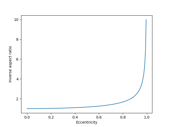
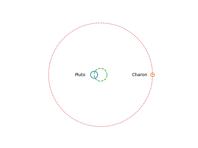
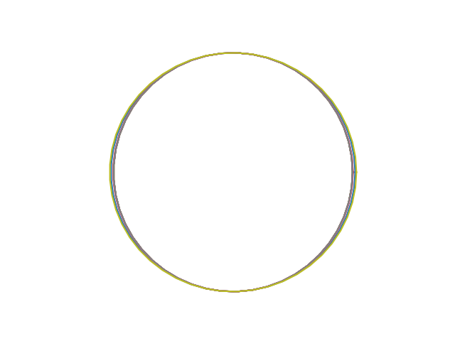
Notice that 1/r hardly changes as e varies between, say, 0 and 0.4. So saying that Pluto has a “highly elliptical” orbit with e = 0.25 does not mean that the shape of its orbit is far from a circle. Here’s a plot of all the planet orbits in our solar system, or all the planet orbits plus the orbit of Pluto if you’d like to be pedantic.

Converting between eccentricity, flattening, and aspect ratio

I made the comment on Twitter that the orbit of the earth around the sun is closer to being an exact circle than the lines of constant longitude are. This means that the fact that the earth’s equatorial bulge is more geometrically significant than the elliptical nature of our orbit.

If you want to confirm this statement, you’ll need to know the shape of earth’s orbit and the shape of a meridian. But you’re most likely to find the former described in terms of eccentricity and the latter in terms of flattening. This is an example of why you might want to convert between different ways of describing the shape of an ellipse. Here are the conversion formulas.

$\begin{align*} e &= \sqrt{2f - f^2} \\ e &= \sqrt{1-r^2} \\ f &= 1-\sqrt{1-e^2} \\ f &= 1-r \\ r &= \sqrt{1-e^2} \\ r &= 1-f \\ \end{align*}$

According to Wikipedia, the eccentricity of earth’s orbit is 0.01671 and the flattening is 1/298.3. To put these on a common scale, meridians have eccentricity: 0.08181, about five times the eccentricity of earth’s orbit.

Similarly, the earth’s orbit has flattening 0.00013962 or about 24 times the flattening of the meridians.

So you could say earth’s orbit is 4 times or 24 times closer to being a circle than earth’s meridians are. The two ratios are very different because the conversion between eccentricity and flattening is highly nonlinear.

Planetary orbits are very nearly circular

Posted on 13 October 2022 by John

If a science book shows you obviously elliptical orbits of planets, it is literally stretching the truth.

I was taught that our benighted ancestors insisted that planetary orbits are circles for philosophical reasons. In fact, they insisted planetary orbits are circular because they very nearly are.

Here’s a plot of the orbits of all nine planets in our solar system, or all eight planets and the dwarf planet Pluto if you prefer, scaled so that they all have the same semi-minor axis.

See how far the “highly elliptical” orbit of Pluto extends past the perfect circle in the inside? Me neither.

Here is how Kepler discovered that planets have elliptical orbits [1].

From 1601 to 1608, he [Kepler] tried fitting various geometrical curves to Tycho’s data on the positions of Mars. Finally, after struggling for almost a year to remove a discrepancy of of 8 minutes of arc (which a less honest man might have chosen to ignore!) Kepler hit upon the ellipse as a possible solution.

It was only by obsessing over a discrepancy of 0.037% of a circle that Kepler was able to discover that Mars has an elliptical orbit.

The next post explains why eccentricity numbers are misleading. The orbit of Pluto, for example, is “highly eccentric” with eccentricity 0.25, but this does not result in an orbit far from circular.

[1] Roger Bate et al. Fundamentals of Astrodynamics. Dover. 1971

Save big money on big queries

Posted on 13 October 2022 by John

server room

I was surprised the first time a client told me that a query would cost them $100,000 to run. If you think about querying a database on your laptop, a long query would take a minute, and what’s the cost of a minute’s worth of electricity? Too small to meter.

But some of my clients have a LOT of data. (Some also come to me with spreadsheets of data.) If you have billions of records hosted in a cloud database like Snowflake, the cost of a query isn’t negligible, especially if it involves complex joins.

There are three ways to reduce the cost of expensive queries.

First of all, it may be possible to solve a different way the problem you’re trying to solve with the expensive query. Maybe the query is the most direct approach but there’s a more economical indirect approach.

Second, it may be possible to rewrite the query into a logically equivalent query that runs faster.

Third, it may be possible to save a tremendous amount of money by tolerating a small probability of error. For example, you may be able to use reservoir sampling rather than an exhaustive query.

This last approach is often misunderstood. Why would you tolerate any chance of error when you could have the exact answer? One reason is that the exact answer might cost 1000x as much to obtain. More importantly, the “exact” result may be the exact answer to a query that is trying estimate something else. The probability of error induced by random sampling may be small relative to the probability of error intrinsic in the problem being solved.

If you’d like me to take a look at how I could reduce your query costs, let’s talk.

The Pluto-Charon orbit

Posted on 13 October 2022 by John

The Moon doesn’t orbit the center of the Earth; it orbits the center of mass of the Earth-Moon system, which is inside the Earth. The distinction matters for designing satellite orbits, but it cannot be seen on a plot to scale. We’ll quantify this below.

Pluto’s moon Charon, however, is so large relative to Pluto and so close, that the center of mass of the Pluto-Charon system is outside of Pluto, and you can easily see this in a plot.

Plot of Pluto and Charon orbiting their barycenter

Imagine Pluto and Charon sitting on each end of a balanced seesaw. Pluto is a distance x₁ to the left of the fulcrum, and Charon is a distance x₂ to the right of the fulcrum. Let m₁ be the mass of Pluto and m₂ be the mass of Charon. Then

m₁ x₁ = m₂ x₂

and

x₁ = m₂ (x₁ + x₂) / (m₁ + m₂).

Now let’s put in some numbers.

m₁ = 1.309 × 10²² kg
m₂ = 1.62 × 10²¹ kg
x₁ + x₂ = 19,640 km

From this we find

x₁ = (1.62 × 19640 / 14.71) km = 2163 km

and so the distance from the center of Pluto to the center of mass of the Pluto-Charon system is 2163 km. But the radius of Pluto is only 1190 km. So the center of mass of the Pluto-Charon system is about as far above the surface of Pluto as the center of Pluto is below the surface.

Comparison with the Earth-Moon system

It matters that the moon doesn’t exactly orbit the center of the Earth, but the difference between the center of the Earth and the center of mass of the Earth-Moon system is less dramatic. Let’s put in the numbers for the Earth and Moon.

m₁ = 5.97 × 10²⁴ kg
m₂ = 7.346 × 10²² kg
x₁ + x₂ = 392,600 km

From this we find

x₁ = (7.346 × 392,600 / 604) km = 4,775 km

The radius of Earth is 6,371 km, and so the center of mass of the Earth-Moon system is inside the Earth.

I made a plot analogous to the one above but for the Earth-Moon system. You could barely see the moon because it is so small relative to the size of its orbit. And you cannot see the difference between the center of the Earth and the barycenter of the Earth and Moon.

Tidal locking

Not only is Charon tidally locked with Pluto, as our moon is with Earth, but Pluto is tidally locked with Charon as well.

On Earth we only ever see one side of the moon. We never see the “dark side,” which is more accurately the “far side.” But someone standing on the moon would see Earth rotate.

Someone standing on Pluto would only ever see one side of Charon, and someone standing on Charon would only ever see one side of Pluto. Sputnik Planitia, the big heart-shaped feature on Pluto, is on the opposite side of Charon, so you could say Pluto is hiding its heart from its companion.

Image of Pluto featuring heart-shaped region

Shape of moon orbit around sun

Posted on 13 October 2022 by John

The earth’s orbit around the sun is nearly a circle, and the moon’s orbit around the earth is nearly a circle, but what is the shape of the moon’s orbit around the sun?

You might expect it to be bumpy, bending inward when the moon is between the earth and the sun and bending output when the moon is on the opposite side of the earth from the sun. But in fact the shape of the moon’s orbit around the sun is convex as proved in [1] and illustrated below.

If the moon orbited the earth much faster, say 10 times faster, at the same altitude, then we see that the orbit is indeed bumpy.

However, the nothing could orbit the earth 10x faster than the moon at the same distance as the moon. Orbital period determines altitude and vice versa.

A more realistic example would be a satellite in MEO (Medium Earth Orbit) like a GPS satellite. Such a satellite orbits the earth roughly twice a day. The path of a MEO satellite around the sun is not convex.

The plot above shows about one day of an MEO satellite’s orbit around the sun. Note that the vertical and horizontal scales are not the same; it would be hard to see anything but a flat line if the scales were the same because the satellite is far closer to the earth than the sun.

Here are the equations from [1]. Choose units so that the distance to the moon or satellite is 1 and let d be the distance from the planet to the sun. Let p be the number of times the moon or satellite orbits the planet as the planet orbits the sun (the number of sidereal periods).

x(θ) = d cos(θ) + cos(pθ)
y(θ) = d sin(θ) + sin(pθ)

This assumes both the planet’s orbit around the sun and the satellite’s orbit around the planet are circular, which is a good approximation in our examples.

[1] Noah Samuel Brannen. The Sun, the Moon, and Convexity. The College Mathematics Journal, Vol. 32, No. 4 (Sep., 2001), pp. 268-272

A more direct approach to series solutions

Posted on 12 October 2022 by John

In the previous post we found a solution to

using operator calculus, i.e. treating the differential operator D like a number and doing tricks with it. See the earlier post for a justification of why we can get away with unorthodox manipulations.

We can generalize the method of the previous post to say that a solution to any differential equation of the form

is given by

$y = \frac{1}{p(D)} f(x).$

In the previous post we had

and

but the method works more generally.

We then find a power series for 1/p(D), most likely by partial fraction decomposition, and apply the result to f(x). There may be a fair amount of labor left, but it’s purely calculus; all the differential equation work is done.

Conceptually, this method subsumes other differential equation techniques such as undetermined coefficients and power series solutions.

Let’s use this method to find an approximate solution to

$y'' + 7y' + 12 = \zeta(x)$

where ζ(x) is the Riemann zeta function.

In the previous post we worked out that

$\frac{1}{D^2 + 7D + 12} = \frac{1}{D+3} - \frac{1}{D+4} = \frac{1}{12} - \frac{7}{144}D + \frac{37}{1728}D^2 + {\cal O}(D^3)$

and so an approximate solution to our differential equation near 0 is

$y(x) = \frac{1}{12}\zeta(0) - \frac{7}{144} \zeta'(0) + \frac{37}{1728}\zeta''(0) + {\cal O}(x^3).$

Numerically this works out to

If you want more terms, carry the series for 1/(D² + 7D + 12) out to more terms.

Operator calculus

Posted on 12 October 2022 by John

Students who take a course in differential equations don’t really learn how to solve differential equations. The problems whose solutions they reproduce were solved over 300 years ago. The methods taught in undergraduate ODE classes are in some sense mnemonics, a way to remember a solution discovered long ago.

Abandon hope of originality

The more scrupulous students in an ODE class cringe at being told “Guess a solution of the form …” because it seems like cheating. They may think “But I really want to learn how to solve things on my own.” This objection isn’t often addressed in part because it’s not often said out loud. But if it were explicitly stated, here’s one way to answer it.

That’s great that you want to learn how to solve differential equations on your own. But solving differential equations, in the sense of finding closed-form solutions by hand, is really hard, and unlikely to succeed. The differential equations that come up in application, that have closed-form solutions, and whose solutions can be calculated by hand in under an hour have been known since the Bernoulli’s. If this is an exaggeration, it’s a slight exaggeration.

You will learn some useful things in this class, and you may even get your first exposure to ideas that latter lead you to do original mathematics [1]. But if so, that original mathematics probably won’t be finding new closed-form solutions to useful differential equations.

This changes the perspective of the ODE class. Instead of pretending that students are going to learn how to solve differential equations ex nihilo, we can be honest that students are going to learn how to “look up” solutions to solved problems. Learning how to look up these solutions is not trivial, and in fact it takes about a semester to learn. You can’t literally look up the solution to a particular differential equation in all its specifics, but you can learn to follow the recipes for classes of equations

The role of rigor

There is a time for everything under the sun. A time for rigor and a time for handwaving. A time to embrace epsilons and a time to shun epsilons.

You can learn a lot of important reusable analysis techniques in the context of differential equations. And if that’s the goal, being rigorous is good. But if the goal is to recall the solution to a solved problem, then it’s expedient to use dirty hacks; think of them almost as mnemonics rather than as solution techniques.

Once you have a candidate solution in hand, you can always rigorously verify that it works by sticking it into the differential equation. In that sense you’re not sacrificing rigor at all.

Operator calculus

Operator calculus treats the differential operator D as a formal symbol and does calculus with it as if it were a number. This is commonly called an abuse of notation, but it has a certain elegance to it. The manipulations could be made rigorous, though not by students in an undergraduate ODE class.

Operator calculus is very powerful, and with great power comes great responsibility. It is not often taught to undergraduates, and for good reason. Sometimes formal operations are justified and sometimes they’re not. Misuse can lead to results that are simply wrong and not just illegally obtained. With that said, let’s jump in.

Let’s find a solution [2] to

Writing the differential operator as D the equation becomes

and so the solution is obviously (!)

$y = \frac{1}{D^2 + 7D + 12} x^2.$

“You can’t just divide by a differential operator like that!” Oh yeah? We’re going to do more than that. We’re going to break it into partial fractions and power series!

$\frac{1}{D^2 + 7D + 12} = \frac{1}{D+3} - \frac{1}{D+4} = \frac{1}{12} - \frac{7}{144}D + \frac{37}{1728}D^2 + {\cal O}(D^3)$

The last term means terms involving D³ and higher powers of D.

Now the first derivative of x² is 2x, the second derivative is 2, and all higher derivatives are 0. So when we apply the operator series above to x² only the terms up to D² contribute anything. From this we can tell that

$\frac{1}{12}x^2 - \frac{7}{72}x + \frac{37}{864}$

is a solution to our differential equation. You may be deeply skeptical of how we got here, and good for you if you are, but it’s easy to show that this is in fact a solution to our differential equation.

Is this worth it?

There are other ways to find a solution to our differential equation. For example, you might have made an inspired guess that the solution is a quadratic polynomial and solved for the coefficients of that polynomial.

On the other hand, the operator calculus approach is more general. We could use a similar approach to solve differential equations with a wide variety of right hand sides. And the approach is systematic enough to be programmed into a computer algebra system.

[1] That was my experience. I specialized in PDEs in grad school and learned a lot that was useful later outside of PDEs.

[2] The general solution to linear equations like this is the general solution to the corresponding homogeneous equation (i.e. with the right hand side set to 0) plus a “particular solution” (i.e. any solution to the equation with the original right hand side restored). Any particular solution will do, because any two particular solutions differ by a solution to the homogeneous equation.

Writing math with Unicode

Posted on 11 October 2022 by John

A LaTeX document looks better than an HTML document, but an HTML document looks better than an awkward hybrid of HTML and inline images created by LaTeX.

My rule is to only use LaTeX-generated images for displayed equations and not for math symbols in the middle of a sentence. This works pretty well, but it’s less than ideal. I use HTML for displayed equations too when I can. Over time I’ve learned how to do more in HTML, and browser support for special characters has improved [1].

My personal prohibition on inline images requires saying in words what I would say in symbols if I were writing LaTeX. For example, in the context of complex variables I have written “z conjugate” rather than put a conjugate bar over z.

There’s a way to fix the particular problem of typesetting conjugates: the Unicode character U+0305 will put a bar (i.e. conjugation symbol) over a character. For example:

If z = a + b i then z̅ − b i.

Here’s the HTML code for the sentence above:

    If <em>z</em> = <em>a</em> + <em>b</em>&#x200a;<em>i</em> 
    then <em>z&#x0305;</em> &#x2212; <em>b</em>&#x200a;<em>i</em>.

Note that the character U+0305, written in HTML as ̅, goes inside the em tags. A couple other things: I put a hair space (U+200A) between b and i, and I used a minus sign (U+2212) rather than a hyphen.

I normally just use a hyphen for a minus sign when I’m blogging about math, but sometimes this doesn’t look right. For example, yesterday’s post about fractional factorial designs had three tables filled with plus signs and minus signs. I first used a hyphen, but that didn’t look right because it was too narrow to visually pair with the plus signs.

Just as you can use U+0305 to put a bar on top of a character, you can use U+20D7 to put a vector on top. For example,

x⃗ = (x₁, x₂, x₃).

This was created with

    <em>x&#x20d7;</em> = (<em>x</em>&#x2081;, 
    <em>x</em>&#x2082;, <em>x</em>&#x2083;).

Here I used the Unicode characters for subscript 1, subscript 2, and subscript 3. Sometimes these look better than <sub>1</sub> etc, but not always. Here’s the equation for x⃗ using sub tags:

x⃗ = (x₁, x₂, x₃).

Unicode typically has all the symbols you need to write mathematics. You can use this page to find the Unicode counterpart to most LaTeX symbols. But text is inherently linear, and you need more than text to lay out typesetting in two dimensions.

Update: Looks like I spoke too soon. The tricks presented here work well on Linux and Mac but not on Windows. Some readers are saying the vector symbol is missing on Windows. On my Windows laptop the bar and vector appear but are not centered over the intended character.

[1] When I started blogging you couldn’t count on browsers having font support for all the mathematical symbols you might want to use. (This post summarizes my experience as of nine years ago.) Now I believe you can, especially for any symbol in the BMP (Basic Multilingual Plane, code points below FFFF). I haven’t gotten feedback from anyone saying they’re missing symbols that I use.

Cicadas and Chicken Nuggets

Posted on 11 October 2022 by John

Yesterday I wrote about the Chicken McNugget problem: if Chicken McNuggets are sold in boxes of 6, 9, and 20, what’s the largest number of nuggets you cannot buy? That post showed that the solution was 43. The technical name for these kinds of problems is numerical monoids.

The method of solution in the previous post is reusable. But before we reuse it, let’s look at a simpler problem involving two units rather than three.

Cicada cycles

Some cicadas appear every 13 years and some every 17 years. So, for example, 43 years from now would be two 13-year cicada cycles and one 17-year cicada cycle. We could ask what the largest number of years is that cannot be expressed in terms of cicada cycles. This is known as the Frobenius number of 13 and 17.

For one thing, there is a largest number of years that cannot be expressed in terms of cicada cycles. If x and y are positive integers, there is an upper bound on the numbers that cannot be expressed as sum of non-negative integer multiples of x and y if and only if x and y are relatively prime. And if x and y are relatively prime, this upper bound is

xy − x − y.

J. J. Sylvester proved this back when Chester A. Arthur was US president [1]. It’s not quite obvious that x and y being relatively prime is sufficient for there to be an upper bound—it follows from Bézout’s lemma—but it is obvious it’s necessary: if x and y are multiples of k > 1, then all sums of integer multiples of x and y are also multiples of k, and so non-multiples of k are unreachable.

So Sylvester’s theorem shows that the Frobenius number of 13 and 17 is 13×17 − 13 − 17 = 191.

Throwing in Venus

Venus goes around the sun 13 times in the time it takes Earth to go around 8 times. That is, Venus and Earth line up every 8 years (from the perspective of our planet). What if we throw in multiples of 8 year cycles? We could, for example, express 25 years as one 17-year cicada cycle and one cycle of Venus.

We know there’s an upper bound on numbers that cannot be expressed as non-negative integer combinations of 13, 17, and 8 because we can express every number greater than 191 using 13 and 17 alone. Adding a new generator cannot increase the Frobenius number. In fact, in this case we know it lowers it because we could apply Sylvester’s theorem to 8 and 13 and show that the Frobenius number of 8, 13, and 17 is at most 83.

Algorithm

There is no analog of Sylvester’s theorem for more than two generators, but we could always compute the Frobenius number in a particular case using the approach from the McNugget post: use brute force up to a point, then use theory to argue that’s enough. In that post, the smallest generator was 6, and we used brute force until we found 6 consecutive numbers that could be produced as non-negative integer combinations of our generators. We could improve on this approach by using Sylvester’s theorem: we use brute force for all combinations that could possibly generate a result lower than an upper bound obtained by Sylvester’s theorem. There are more efficient algorithms—see [2] for references—but the following will work.

    from math import gcd, floor
    from itertools import product

    def frobenius(generators):
        "assumes the smallest two generators are relatively prime"
        g = sorted(generators)
        assert(len(g) > 1)
        assert(gcd(g[0], g[1]) == 1)
        ub = g[0]*g[1] 
        
        limits = [range(int(floor(ub/n))) for n in generators]
        reachable = set()
        for p in product(*limits):
            combo = sum(p[i]*g[i] for i in range(len(g)))
            if combo < ub:
                reachable.add(combo)
        complement = set(range(ub)) - reachable
        return(max(complement))
    
    print( frobenius([13, 17, 8]) )

This shows that the Frobenius number of 8, 13, and 17 is 44.

Just to do another example, the code can show that the smallest number of days not representable by multiples of 7, 30, and 365 is 209 days.

Notes

[1] J. J. Sylvester, Mathematical questions with their solutions, Educational Times 41 (1884) 171–178.

[2] Factoring in the Chicken McNugget monoid. arXiv:1709.01606

The Chicken McNugget Monoid

Posted on 10 October 2022 by John

When McDonalds first introduced Chicken McNuggets, you could buy McNuggets in boxes of 6, 9, or 20. The Chicken McNugget problem is to determine which numbers of McNuggets you can and cannot buy. A number n is a McNugget number if it is possible to buy exactly that many McNuggets (using the original boxes).

Box of 6 Chicken McNuggets

There are only finitely many non-McNugget numbers, and these are listed in OEIS sequence A065003.

Note that if you order eight boxes of 6 nuggets you get 48 nuggets, and so if you order more than eight boxes, in any combination, you get more than 48 nuggets. So the following program will compute all McNugget numbers less than 48.

    ns = set() 
    for i in range(8):
        for j in range(8):
            for k in range(8):
                n = 6*i + 9*j + 20*k
                if n <= 48:
                    ns.add(n)
    
    comp = set(range(48)) - ns

The non-McNugget numbers less than 48 are stored in comp, the set complement of ns. These numbers are

1, 2, 3, 4, 5, 7, 8, 10, 11, 13, 14, 16, 17, 19, 22, 23, 25, 28, 31, 34, 37, 43.

It turns out 48 and 49 are also McNugget numbers. You can verify this by changing “48” to “50” in the code above and looking at ns. This means that 44, 45, 46, 47, 48, and 49, a run of 6 consecutive numbers are all McNugget numbers, and so you can add boxes of 6 to these numbers to get any greater number. This shows that 43 is the largest non-McNugget number.

The set of McNugget numbers contains 0, my favorite number of McNuggets, and is closed under addition, and so it forms a monoid.

Update: The next post generalizes this one, giving a little theory and more general code.

Source: Factoring in the Chicken McNugget monoid. arXiv:1709.01606

Month: October 2022

Eccentricity, Flattening, and Aspect Ratio

Converting between eccentricity, flattening, and aspect ratio

Related posts

Planetary orbits are very nearly circular

Save big money on big queries

Related posts

The Pluto-Charon orbit

Comparison with the Earth-Moon system

Tidal locking

More orbital mechanics posts

Shape of moon orbit around sun

A more direct approach to series solutions

Related links

Operator calculus

Abandon hope of originality

The role of rigor

Operator calculus

Is this worth it?

Related posts

Writing math with Unicode

Related posts

Cicadas and Chicken Nuggets

Cicada cycles

Throwing in Venus

Algorithm

Notes

The Chicken McNugget Monoid