Suppose you have a mass suspended by the combination of a spring and a rubber band. A spring resists being compressed but a rubber band does not. So the rubber band resists motion as the mass moves down but not as it moves up. In [1] the authors use this situation to motivate the following differential equation:
![]()
where
![]()
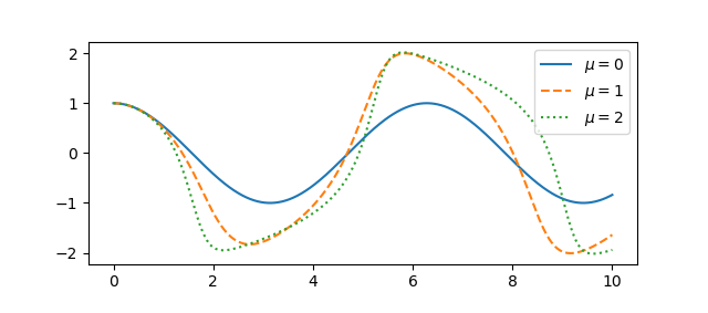
If a = b then we have a linear equation, an ordinary damped, driven harmonic oscillator. But the asymmetry of the behavior of the rubber band causes a and b to be unequal, and that’s what makes the solutions interesting.
For some parameters the system exhibits essentially sinusoidal behavior, but for other parameters the behavior can become chaotic.
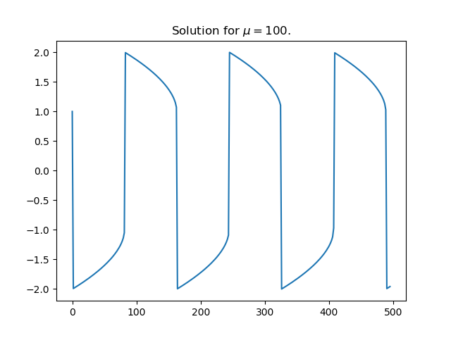
Here’s an example of complex behavior.
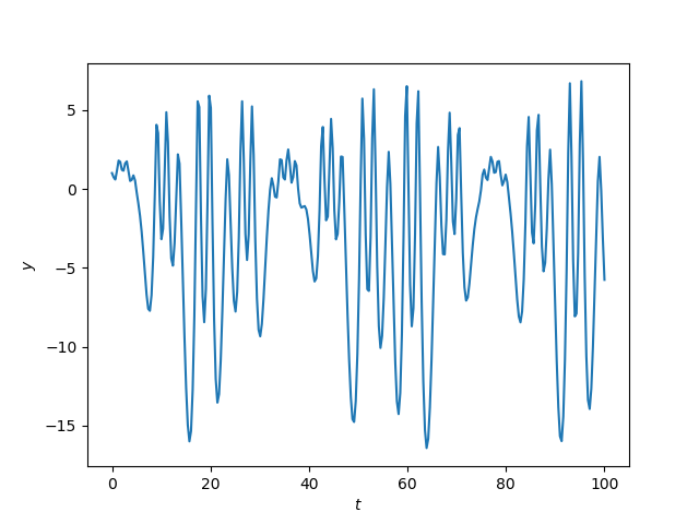
Here’s the Python code that produced the plot.
    from scipy import linspace, sin
    from scipy.integrate import solve_ivp
    import matplotlib.pyplot as plt

    def pos(x):
        return max(x, 0)

    def neg(x):
        return max(-x, 0)

    a, b, λ, μ = 17, 1, 15.4, 0.75

    def system(t, z):
        y, yp = z # yp = y'
        return [yp, 10 + λ*sin(μ*t) - 0.01*yp - a*pos(y) + b*neg(y)]

    t = linspace(0, 100, 300)

    sol = solve_ivp(system, [0, 100], [1, 0], t_eval=t)
    plt.plot(sol.t, sol.y[0])
    plt.xlabel("$t$")
    plt.ylabel("$y$")
In a recent post I said that I never use non-ASCII characters in programming, so in the code above I did. In particular, it was nice to use λ as a variable; you can’t use lambda as a variable name because it’s a reserved keyword in Python.
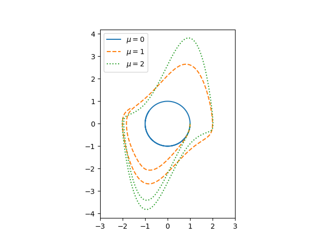
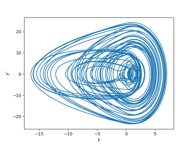
Update: Here’s a phase portrait for the same system.
More posts on differential equations
- Ten life lessons from differential equations
- Maximum principles for boundary value problems
- Self-curvature
[1] L. D. Humphreys and R. Shammas. Finding Unpredictable Behavior in a Simple Ordinary Differential Equation. The College Mathematics Journal, Vol. 31, No. 5 (Nov., 2000), pp. 338-346