Time to factor big integers Python and Mathematica

This post will look at the time required to factor n − 1 each of the following prime numbers in Python (SymPy) and Mathematica. The next post will explain why I wanted to factor these numbers.

p = 2254 + 4707489544292117082687961190295928833
q = 2254 + 4707489545178046908921067385359695873
r = 2254 + 45560315531419706090280762371685220353
s = 2254 + 45560315531506369815346746415080538113

Here are the timing results.

    |   |   Python | Mathematica |
    |---+----------+-------------|
    | p |    0.913 |       0.616 |
    | q |    0.003 |       0.002 |
    | r |  582.107 |      14.915 |
    | s | 1065.925 |      20.763 |

This is hardly a carefully designed benchmark, but it’s enough to suggest Mathematica can be a couple orders of magnitude faster than Python.

Here are the factorizations.

p − 1 = 234 × 3 × 4322432633228119 × 129942003317277863333406104563609448670518081918257
q − 1 = 233 × 3 × 5179 × 216901160674121772178243990852639108850176422522235334586122689
r − 1 = 232 × 32 × 463 × 539204044132271846773 × 8999194758858563409123804352480028797519453
s − 1 = 232 × 32 × 1709 × 24859 × 1690502597179744445941507 × 10427374428728808478656897599072717

Powers of 3 + √2

Yesterday’s post looked at the distribution of powers of x mod 1. For almost all x > 1 the distribution is uniform in the limit. But there are exceptions, and the post raised the question of whether 3 + √2 is an exception.

A plot made it look like 3 + √2 is an exception, but that turned out to be a numerical problem.

A higher precision calculation showed that the zeros on the right end of the plot were erroneous.

So this raises the question of how to calculate (3 + √2)n accurately for large n. The way I created the second plot was to use bc to numerically calculate the powers of 3 + √2. In this post, I’ll look at using Mathematica to calculate the powers symbolically.

For all positive integers n,

(3 + √2)n = an + bn√2

where an and bn are positive integers. We want to compute the a and b values.

If you ask Mathematica to compute (3 + √2)n it will simply echo the expression. But if you use the Expand function it will give you want. For example

    Expand[(3 + Sqrt[2])^10]

returns

    1404491 + 993054 √2

We can use the Coefficient function to split a + b √2 into a and b.

    parts[n_] := 
        Module[{x = (3 + Sqrt[2])^n}, 
            {Coefficient[x, Sqrt[2], 0], Coefficient[x, Sqrt[2], 1]}]

Now parts[10] returns the pair {1404491, 993054}.

Here’s something interesting. If we set

(3 + √2)n = an + bn√2

as above, then the two halves of the expression on the right are asymptotically equal. That is, as n goes to infinity, the ratio

anbn√2

converges to 1.

We can see this by defining

    ratio[n_] := 
        Module[ {a = Part[ parts[n], 1], b = Part[parts[n], 2]}, 
        N[a / (b Sqrt[2])]]

and evaluating ratio at increasing values of n. ratio[12] returns 1.00001 and ratio[13] returns 1, not that the ratio is exactly 1, but it is as close to 1 as a floating point number can represent.

This seems to be true more generally, as we can investigate with the following function.

    ratio2[p_, q_, r_, n_] := 
        Module[{x = (p + q Sqrt[r])^n}, 
            N[Coefficient[x, Sqrt[r], 0]/(Coefficient[x, Sqrt[r], 1] Sqrt[r])]]

When r is a prime and

(p + q√r)n = an + bnr

then it seems that the ratio an / bnr converges to 1 as n goes to infinity. For example, ratio2[3, 5, 11, 40] returns 1, meaning that the two halves of the expression for (3 + 5√11)n are asymptotically equal.

I don’t know whether the suggested result is true, or how to prove it if it is true. Feels like a result from algebraic number theory, which is not something I know much about.

Update: An anonymous person on X suggested a clever and simple proof. Observe that

\begin{align*} a_n &= \frac{(3+\sqrt{2})^n + (3-\sqrt{2})^n}{2} \\ b_n\sqrt{2} &= \frac{(3 + \sqrt{2})^n - (3-\sqrt{2})^n}{2} \end{align*}

In this form it’s clear that the ratio an / bn √2 converges to 1, and the proof can be generalized to cover more.

How Mathematica Draws a Dragonfly

Mathematica includes code to draw various whimsical images. For example, if you enter the following command in Mathematica

    Entity["PopularCurve", "DragonflyCurve"][
        EntityProperty["PopularCurve", "Image"]]

you get an image of a dragonfly.

It draws such images with Fourier series. You can tell by asking for the parameterization of the curve. If you enter

    Entity["PopularCurve", "DragonflyCurve"][
        EntityProperty["PopularCurve", "ParametricEquations"]]

you’ll get the following, after some rearrangement.

    Function[t, {
        (7714/27) Sin[47/20 - t] + (1527/37) Sin[16/5 - 2t] + 
        (3202/39) Sin[108/41 - 3t] + … + 2/9 Sin[15/19 - 81 t], 
        (9406/37) Sin[29/7 - t] + (3591/53) Sin[28/13 - 2t] + 
        (1111/20) Sin[9/23 - 3t] + … -(3/29) Sin[8/23 + 81 t]
        }]

The function is a parameterized curve, taking t to (x(t), y(t)) where x(t) and y(t) are Fourier series including frequencies up to sin(81t). Each of the sine terms has a phase shift that could be eliminated by expressing sin(φ + ωt) as a linear combination of sin(ωt) and cos(ωt).

Presumably somebody drew the dragonfly, say in Adobe Illustrator or Inkscape, then did a Fourier transform of a sampling of the curve.

To make sure Mathematica wasn’t doing anything behind the scenes that I wasn’t aware of, I reproduced the dragonfly curve by porting the Mathematica code to Python.

The number of Fourier components needed to draw an image depends on the smoothness and complexity of the image. The curve for π, for example, the highest frequency component is sin(32t).

The triceratops curve is more complicated and Mathematica uses frequencies up to sin(188t).


n-queens in 3D

It’s possible to place n queens on an n × n chess board so that no queen is attacking any other queen, provided n > 3. A queen is able to move any number of squares in any horizontal, vertical, or diagonal direction. Another way to put it is that the queen can move in any of 8 = 3² − 1 directions, in the direction of any cell in a 3 × 3 grid centered on the queen.

What if we extend chess to three dimensions? Now we have an n × n × n cube. Now a queen is able to move in 26 = 3³ − 1 directions, in the direction of any cell in a 3 × 3 × 3 cube centered on the queen.

Klarner [1] proved that it is possible to place n² queens in an n × n × n cube so that no queen is attacking any other, provided gcd(n, 210) = 1, i.e. provided the smallest prime factor of n is larger than 7. The condition gcd(n, 210) = 1 is sufficient, and it is conjectured to be necessary as well [2].

Klarner constructed a solution as follows: Place the queens on

(ij, (3i + 5j) mod n)

for i and j running from 1 to n.

One way to visualize the queens in 3D is to draw a 2D grid where each cell contains the vertical coordinate of the corresponding queen. This grid will be a Latin square, and so the 3D queen placement problem is also known as the Latin queen problem.

Here’s a visualization of Klarner’s example.

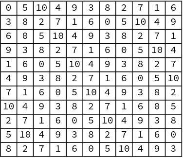
Note that if you only pay attention to a particular number, you have a solution to the 11 queens problem in a square. That’s because every slice of a 3D solution is a solution to the 2D problem.

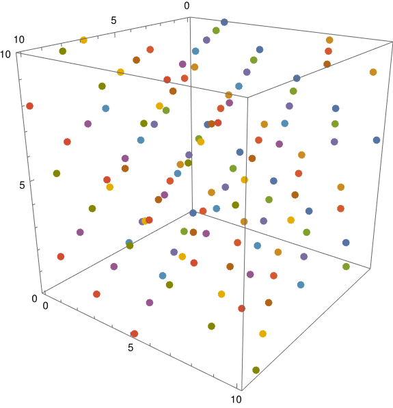
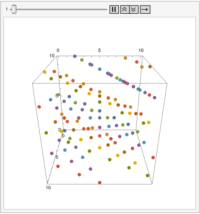
I played around with plotting the points in three dimensions. Here’s one view.

A slight rotation of the cube gives a substantially different perspective. This would be better as an animation, available here.

Mathematica code

Here’s the code that made the images above.

Flat grid:

    Grid[
        Table[
            Mod[3 i + 5 j, 11], 
            {i, 0, 10}, 
            {j, 0, 10}
        ], 
        Frame -> All
    ]

Static 3D view:

     ListPointPlot3D[
         Table[
             {i, j, Mod[3 i + 5 j, 11]}, 
             {i, 0, 10}, 
             {j, 0, 10}
          ], 
          BoxRatios -> {1, 1, 1}, 
          PlotStyle -> {PointSize[0.02]}
      ]

Animation:

    Animate[
        ListPointPlot3D[
            Table[
                {i, j, Mod[3 i + 5 j, 11]}, 
                {i, 0, 10}, 
                {j, 0, 10}
            ], 
        BoxRatios -> {1, 1, 1}, 
        PlotStyle -> {PointSize[0.02]}, 
        ViewPoint -> {2 Cos[t], 2 Sin[t], 1}
        ], 
        {t, 0, Pi, 0.05}, 
        AnimationRunning -> True, 
        AnimationRate -> 4
    ]

    Export["klerner_animation.gif", %]

Related posts

[1] D.A. Klarner, Queen squares, J. Recreational Math. 12 (3) (1979/1980) 177–178.

[2] Jordan Bell and Brett Stevens. A survey of known results and research areas for n-queens. Discrete Mathematics 309 (2009) 1–31

Duplicating a hand-drawn contour plot

Like the previous post, this post also seeks to approximately reproduce a hand-drawn plot. This time the goal is reproduce figure 7.3 from A&S page 298.

This plot is a visualizing of the function of a complex variable

w(z) = exp(−z²) erfc(− iz)

where erfc is the complementary error function.

A&S calls the graph above an “altitude chart.” This could be a little misleading since it’s the overlay of two plots. One plot is the absolute value of w(z), which could well be called altitude. But it also contains a plot of the phase. To put it another way, if we denote the values of the function in polar form r exp(iθ) the altitude chart is an overlay of a plot of r and a plot of θ.

We begin by defining

f[z_] := Exp[-z^2] Erfc[-I z]

The following code reproduces the lines of constant phase fairly well.

ContourPlot[Arg[f[x + I y]], {x, 0.1, 3.1}, {y, -2.5, 3}, 
    Contours -> 20, ContourShading -> None, AspectRatio -> 1.6]

The lines of constant absolute value take a little more effort to reproduce. If we let Mathematica pick where to put the contour lines, they will not be distributed the same way they were in A&S.

ContourPlot[Abs[f[x + I y]], {x, 0, 3.1}, {y, -2.6, 3}, 
    Contours -> 20, ContourShading -> None, AspectRatio -> 1.6]

We can duplicated the spacing in the original plot by providing Mathematica a list of contour values rather than number of contour values.

ContourPlot[Abs[f[x + I y]], {x, 0, 3.1}, {y, -2.6, 3}, 
    Contours -> {0.2, 0.3, 0.4, 0.5, 0.6, 0.7, 0.8, 0.9, 1, 2, 3, 4, 5, 10, 100}, 
    ContourShading -> None, AspectRatio -> 1.6]

(For reasons I don’t understand, Mathematica does not draw the contours corresponding to w = 10 and w = 100.)

When I overlay the phase and absolute value plots with the Show command I get a plot approximately reproducing the original.

Related posts

Reproducing a hand-drawn plot

The plots in old (i.e. pre-computer) math books are impressive. These plots took a lot of effort to produce, and so they weren’t created lightly. Consequently they tend to be aesthetically and mathematically interesting. A few weeks ago I recreated a plot from A&S using Mathematica, and today I’d like to do the same for the plot below from a different source [1].

Here is my approximate reproduction.

I’ll give the mathematical details below for those who are interested.

The plot shows “normalized associated Legendre functions of the first kind.” There are two families of Legendre polynomials, denoted P and Q; we’re interested in the former. “Associated” means polynomials that are derived the Legendre polynomials by taking derivatives. Normalized means the polynomials are multiplied by constants so that their squares integrate to 1 over [−1, 1].

Mathematica has a function LegendreP[n, m, x] that implements the associated Legendre polynomials Pnm(x). I didn’t see that Mathematica has a function for the normalized version of these functions, so I rolled by own.

f[n_, m_, x_] := (-1)^n LegendreP[n, m, x] 
        Sqrt[(2 n + 1) Factorial[n - m]/(2 Factorial[n + m])]

I added the alternating sign term up front after discovering that apparently the original plot used a different convention for defining Pnm than Mathematica uses.

I make my plot by stacking the plots created by

Plot[Table[f[n, n, x], {n, 1, 8}],  {x, 0, 1}]

and

Plot[Table[f[n + 4, n, x], {n, 0, 4}],  {x, 0, 1}]

The original plot shows P4(x). I used the fact that this equals P40(x) to simplify the code. I also left out the flat line plotting P0 because I thought that looked better.

Related post: Duplicating a Hankel function plot from A&S.

[1] Tables Of Functions With Formulae And Curves by Fritz Emde, published in 1945. Available on Archive.org.

Duplicating Hankel plot from A&S

Abramowitz and Stegun has quite a few intriguing plots. The post will focus on the follow plot, Figure 9.4, available here.

A&S figure 9.4

We will explain what the plot is and approximately reproduce it.

The plot comes from the chapter on Bessel functions, but the caption says it is a plot of the Hankel function H0(1). Why a plot of a Hankel function and not a Bessel function? The Hankel functions are linear combinations of the Bessel functions of the first and second kind:

H0(1) = J0i Y0

More on that Hankel functions and their relations to Bessel functions here.

The plot is the overlay of two kinds of contour plots: one for lines of constant magnitude and one for lines of constant phase. That is, if the function values are written in the form reiθ then one plot shows lines of constant r and one plot shows lines of constant θ.

We can roughly reproduce the plot of magnitude contours with the following Mathematica command:

ContourPlot[Abs[HankelH1[0, x + I y]], {x, -4, 2 }, {y, -1.5 , 1.5 }, 
 Contours -> 20, ContourShading -> None, AspectRatio -> 1/2]

This produces the following plot.

Absolute value contour

Similarly, we can replace Abs with Arg in the Mathematica command and increase Contours to 30 to obtain the following phase contour plot.

Phase contour

Finally, we can stack the two plots on top of each other using Mathematica’s Show command.

Magnitude and phase contours

By the way, you can clearly see the branch cut in the middle. The Hankel function is continuous (even analytic) as you move clockwise from the second quadrant around to the third, but it is discontinuous across the negative real axis because of the branch cut.

Related posts

Constellations in Mathematica

Mathematica has data on stars and constellations. Here is Mathematica code to create a list of constellations, sorted by the declination (essentially latitude on the celestial sphere) of the brightest star in the constellation.

constellations = EntityList["Constellation"]
sorted = SortBy[constellations, -#["BrightStars"][[1]]["Declination"] &]

We can print the name of each constellation with

Map[#["Name"] &, sorted]

This yields

{"Ursa Minor", "Cepheus", "Cassiopeia", "Camelopardalis", 
…, "Hydrus", "Octans", "Apus"}

We can print the name of the constellation along with its brightest star as follows.

Scan[Print[#["Name"], ", " #["BrightStars"][[1]]["Name"]] &, sorted]

This prints

Ursa Minor, Polaris
Cepheus, Alderamin
Cassiopeia, Tsih
Camelopardalis, β Camelopardalis
…
Hydrus, β Hydri
Octans, ν Octantis
Apus, α Apodis

Mathematica can draw star charts for constellations, but when I tried

Entity["Constellation", "Orion"]["ConstellationGraphic"]

it produced extraneous text on top of the graphic.

Related posts

A disk around Paris

The other day I saw an image of a large disk centered on Paris subjected to the Mercator projection. I was playing around in Mathematica and made similar images for different projections. Each image below is a disk of radius 4200 km centered on Paris (latitude 49°, longitude 2°).

All images were produced with the following Mathematica code, changing the GeoProjection argument each time.

    GeoGraphics[GeoDisk[GeoPosition[{49, 2}],
       Quantity[4200, "Kilometers"] ],
       GeoProjection -> "...", 
       GeoRange -> "World"]

Robinson projection

    … GeoProjection -> "Robinson", …

Robinson projection

Winkel-Snyder projection

    … GeoProjection -> "WinkelSnyder", …

Winkel-Snyder projection

Orthographic projection

    … GeoProjection -> "Orthographic", …

Orthographic projection

Lambert Azimuthal projection

    … GeoProjection -> "LambertAzimuthal", …

Lambert Azimuthal projection

Peirce Quincuncial projection

    … GeoProjection -> "PeirceQuincuncial", …

Peirce Quincuncial projection

This last projection has some interesting mathematics and history behind it. See this post for the backstory.

Curvature: principal, Gauss, and mean

This post will compute the center of curvature for an object described in the previous post. In order to do that we first need to describe principle curvature and Gauss curvature, and we’ll throw in mean curvature while we’re at it.

Let S be a surface sitting in three dimensional space. No need for more generality to get where we want to go. At any point p on S we can draw curves on the S through p and compute the curvature at p. The curvature is the reciprocal of the radius of the kissing circle.

If we draw curves through p in every direction, some may have larger or smaller curvature than others. Let k1 and k2 be the minimum and maximum curvatures at p. These re the principal curvatures. The product k1 k2 of the principle curvatures is the Gaussian curvature and their average ( k1 + k2)/2 is the mean curvature. Incidentally, when principle curvatures are not equal. the directions in which the curvature is minimized and maximized are orthogonal.

In the previous post I said that the center of curvature for the surface with equation

x^2 + y^2 + (z/h)^2 = s^2 (x^2 + y^2) (z/h)^2 + 1

is finite because the curvature is always positive. In particular, we wanted to know the center of curvature at the bottom, where x = y = 0 and z = −h.

The calculation to get there is messy, but the end result is simple: the principle curvatures are equal by symmetry, and both equal 1 − s². Therefore the center of curvature is at z = 1/(1 − s²).

Calculation details

The following Mathematica code calculates the (signed) curvature of a curve of the form F(x, y) = 0.

k[f_, x_, y_] := (D[f[x, y], y]^2 D[f[x, y], {x, 2}] - 
    2 D[f[x, y], x] D[f[x, y], y] D[f[x, y], {x, 1}, {y, 1}] + 
    D[f[x, y], x]^2 D[f[x, y], {y, 2}]) / (D[f[x, y], x]^2 + 
     D[f[x, y], y]^2)^(3/2)

Define

g[x_, y_] := x^2 + y^2 - s^2 x^2 y^1 - 1

and replace y with z/h. When we evaluate the curvature at x = 0 and simplify

Simplify[k[g, x, y] /. { y -> z/h, x -> 0}, Assumptions -> {h > 0}]

we get

(hs² z) / |z|.

When z = −h we find that the unsigned curvature is 1 − s². In the previous post we assumed h > 1, but the calculation above shows that if h < 1 it’s possible for the curvature to be 0. (Recall s must be between 0 and 1.)

Related posts