I was flipping through Gravitation [1] this weekend and was curious about an illustration on page 309. This post reproduces that graph.
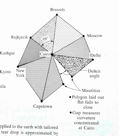
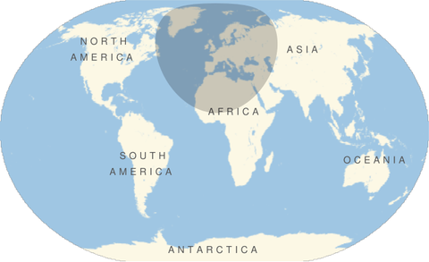
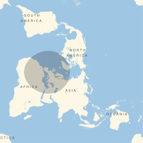
The graph is centered at Cairo, Egypt and includes triangles whose side lengths are the distances between cities. The triangles are calculated using only distances, not by measuring angles per se.
The geometry of each triangle is Euclidean: giving the three edge lengths fixes all the features of the figure, including the indicated angle. … The triangles that belong to a given vertex [i.e. Cairo], laid out on a flat surface, fail to meet.
I will reproduce the plot in Python because I’m more familiar with making plots there. But I’ll get the geographic data out of Mathematica, because I know how to do that there.
Geographic information from Mathematica
I found the distances between the various cities using the GeoDistance function in Mathematica. The arguments to GeoDistance are “entities” which are a bit opaque. When using Mathematica interactively, you can use ctrl + = to enter the name of an entity. There’s some guesswork, e.g. whether I meant New York City or the state of New York when I entered “New York”, but Mathematica guessed correctly. The following code lists the city entities explicitly.
    cities = {
        Entity["City", {"Cairo", "Cairo", "Egypt"}],
        Entity["City", {"Delhi", "Delhi", "India"}],
        Entity["City", {"Moscow", "Moscow", "Russia"}],
        Entity["City", {"Brussels", "Brussels", "Belgium"}],
        Entity["City", {"Reykjavik", "Hofudhborgarsvaedhi", "Iceland"}],
        Entity["City", {"NewYork", "NewYork", "UnitedStates"}],
        Entity["City", {"CapeTown", "WesternCape", "SouthAfrica"}],
        Entity["City", {"PortLouis", "PortLouis", "Mauritius"}] }
Most of these are predictable, but I would not have guessed the code for Reykjavik or Cape Town. I found these by using the command InputForm and entering the entities as above.
I found the distance from Cairo to each of the other cities with
Table[GeoDistance[cities[[1]], cities[[i]]], {i, 2, 8}]
and the distances from the cities to their neighbors with
    Table[GeoDistance[cities[[i]], cities[[i + 1]]], {i, 2, 7}]
    GeoDistance[cities[[8]], cities[[2]]]
Drawing the plot
Now that we’ve got the data, how do we draw the plot?
Let’s put Cairo at the origin. First we draw a line from Cairo to Delhi. We might as well put Delhi on the x-axis to make things simple.
Next we need to plot Moscow. We know the distance R1 from Cairo to Moscow, and the distance R2 from Delhi to Moscow. So imagine drawing a circle of radius R1 centered at Cairo and a circle of radius R1 centered at Delhi. Moscow is located where the two circles intersect. The previous post shows how to find the intersection of circles.
The two circles intersect in at two points, so which do we choose? We choose the intersection point that preserves the orientation of the original graph (and the globe). As we go through the cities in counterclockwise order, the cross product of the previous line to the next line should have positive z component.
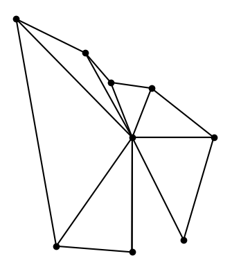
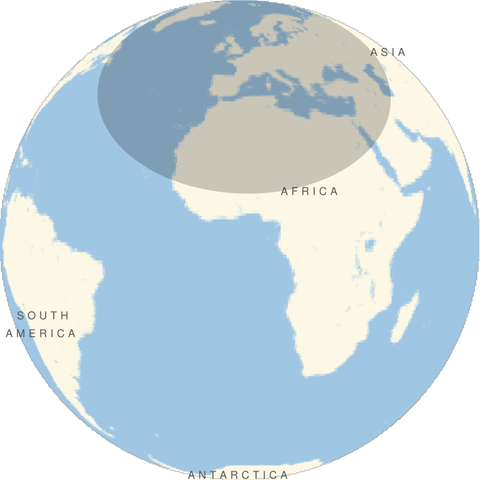
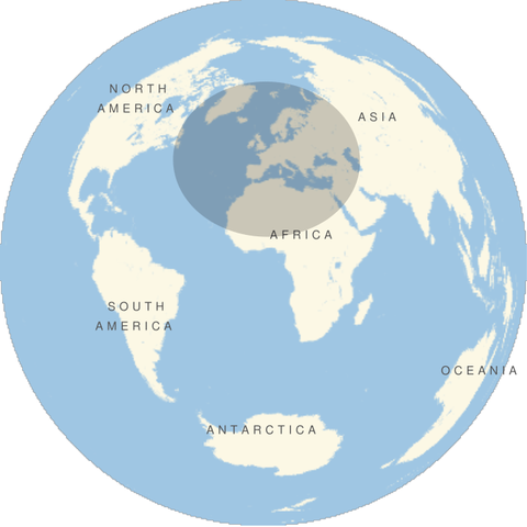
This shows that the original graph was not to scale, though the gap between triangles was approximately to scale. In hindsight this should have been obvious: Brussels and Reykjavik are much closer to each other than Capetown and New York are.
The gap
Why the gap? Because the earth is curved at Cairo (and everywhere else). If the earth were flat, the triangles would fit together without any gaps.
There’s no gap when you take spherical triangles on the globe. But even though the triangles preserve length when projected to the plane, they cannot preserve angles too. The sum of the angles in a spherical triangle adds up to more than 180°, and the amount by which the sum exceeds 180° is proportional to the size of the spherical triangle. Since the angles of triangles in the plane do add up to 180°, each flat triangle fails to capture a bit of the corresponding spherical triangles, and the failures add up to the gap we see in the image.
[1] Gravitation by Misner, Thorne, and Wheeler. 1973.