How to digitize a graph

Suppose you have a graph of a function, but you don’t have an equation for it or the data that produced it. How can you reconstruction the function?

There are a lot of software packages to digitize images. For example, Web Plot Digitizer is one you can use online. Once you have digitized the graph at a few points, you can fit a spline to the points to approximately reconstruct the function. Then as a sanity check, plot your reconstruction to see if it looks like the original. It helps to have the same aspect ratio so you’re not distracted by something that doesn’t matter, and so that differences that do matter are easier to see.

For example, here is a graph from Zwicker and Fastl’s book on psychoacoustics. It contains many graphs with no data or formulas. This particular one gives the logarithmic transmission factor between free field and the peripheral hearing system.

Here’s Python code to reconstruct the functions behind these two curves.

import matplotlib.pyplot as plt
import numpy as np
from scipy import interpolate 

curve_names = ["Free", "Diffuse"]
plot_styles = { "Free" : 'b-', "Diffuse" : 'g:'}

data = {}
for name in curve_names:
    data = np.loadtxt("{}.csv".format(name), delimiter=',')

    x = data[:,0]
    y = data[:,1]
    spline = interpolate.splrep(x, y)
    xnew = np.linspace(0, max(x), 100)
    ynew = interpolate.splev(xnew, spline, der=0)
    plt.plot(xnew, ynew, plot_styles[name])
 
logical_x_range  = 24    # Bark
logical_y_range  = 40    # dB
physical_x_range = 7     # inch
physical_y_range = 1.625 # inch

plt.legend(curve_names, loc=2)
plt.xlabel("critical-band rate")
plt.ylabel("attenuation")
plt.xlim((0, logical_x_range))


plt.axes().set_aspect( 
    (physical_y_range/logical_y_range) / 
    (physical_x_range/logical_x_range) )
ax = plt.gca()
ax.get_xaxis().set_ticks([0, 4, 8, 12, 16, 20, 24])
ax.get_yaxis().set_ticks([-10, 0, 10, 20, 30])

plt.show()

Here’s the reconstructed graph.

Cornu’s spiral

Cornu’s spiral is the curve parameterized by

x(t) = C(t) = \int_0^t \cos \left( \frac{\pi}{2} s^2 \right) \, ds \\ y(t) = S(t) = \int_0^t \sin \left( \frac{\pi}{2} s^2 \right) \, ds

where C and S are the Fresnel functions, sometimes called the Fresnel cosine integral and Fresnel sine integral. Here’s a plot of the spiral.

Cornu's spiral

Both Fresnel functions approach ½ as t → ∞ and so the curve slowly spirals toward (½, ½) in the first quadrant. And by symmetry, because both functions are odd, the curve spirals toward (-½, -½) in the third quadrant.

Here’s the Python code used to make the plot.

    from scipy.special import fresnel
    from scipy import linspace
    import matplotlib.pyplot as plt

    t = linspace(-7, 7, 1000)
    y, x = fresnel(t)

    plt.plot(x, y)
    plt.axes().set_aspect("equal")
    plt.show()

The SciPy function fresnel returns both Fresnel functions at the same time. It returns them in the order (S, C) so the code reverses the order of these to match the Cornu curve.

One interesting feature of Cornu’s spiral is that its curvature increases linearly with time. This is easy to verify: because of the fundamental theorem of calculus, the Fresnel functions reduce to sines and cosines when you take derivatives, and you can show that the curvature at time t equals πt.

How fast does the curve spiral toward (½, ½)? Since the curvature at time t is πt, that says that at time t the curve is instantaneously bending like a circle of radius 1/πt. So the radius of the spiral is decreasing like 1/πt.

Cornu’s spiral was actually discovered by Euler. Cornu was an engineer who independently discovered the curve much later. Perhaps because Cornu used the curve in applications, his name is more commonly associated with the curve. At least I’ve more often seen it named after Cornu. This is an example of Stigler’s law that things are usually not named after the first person to discover them.

Creating police siren sounds with frequency modulation

Yesterday I was looking into calculating fluctuation strength and playing around with some examples. Along the way I discovered how to create files that sound like police sirens. These are sounds with high fluctuation strength.

police car lights

The Python code below starts with a carrier wave at fc = 1500 Hz. Not surprisingly, this frequency is near where hearing is most sensitive. Then this signal is modulated with a signal with frequency fm. This frequency determines the frequency of the fluctuations.

The slower example produced by the code below sounds like a police siren. The faster example makes me think more of an ambulance or fire truck. Next time I hear an emergency vehicle I’ll pay more attention.

If you use a larger value of the modulation index β and a smaller value of the modulation frequency fm you can make a sound like someone tuning a radio, which is no coincidence.

Here are the output audio files in .wav format:

slow.wav

fast.wav

from scipy.io.wavfile import write
from numpy import arange, pi, sin, int16

def f(t, f_c, f_m, beta):
    # t    = time
    # f_c  = carrier frequency
    # f_m  = modulation frequency
    # beta = modulation index
    return sin(2*pi*f_c*t - beta*sin(2*f_m*pi*t))

def to_integer(signal):
    # Take samples in [-1, 1] and scale to 16-bit integers,
    # values between -2^15 and 2^15 - 1.
    return int16(signal*(2**15 - 1))

N = 48000 # samples per second
x = arange(3*N) # three seconds of audio

data = f(x/N, 1500, 2, 100)
write("slow.wav", N, to_integer(data))

data = f(x/N, 1500, 8, 100)
write("fast.wav", N, to_integer(data))

More frequency modulation posts

Graphs and square roots modulo a prime

Imagine a clock with a prime number of hours. So instead of being divided into 12 hours, it might be divided into 11 or 13, for example. You can add numbers on this clock the way you’d add numbers on an ordinary clock: add the two numbers as ordinary integers and take the remainder by p, the number of hours on the clock. You can multiply them the same way: multiply as ordinary integers, then take the remainder by p. This is called arithmetic modulo p, or just mod p.

Which numbers have square roots mod p? That is, for which numbers x does there exist a number y such that y2 = x mod p? It turns out that of the non-zero numbers, half have a square root and half don’t. The numbers that have square roots are called quadratic residues and the ones that do not have square roots are called quadratic nonresidues. Zero is usually left out of the conversation. For example, if you square the numbers 1 through 6 and take the remainder mod 7, you get 1, 4, 2, 2, 4, and 1. So mod 7 the quadratic residues are 1, 2, and 4, and the nonresidues are 3, 5, and 6.

A simple, brute force way to tell whether a number is a quadratic residue mod p is to square all the numbers from 1 to p − 1 and see if any of the results equals your number. There are more efficient algorithms, but this is the easiest to understand.

At first it seems that the quadratic residues and nonresidues are scattered randomly. For example, here are the quadratic residues mod 23:

[1, 2, 3, 4, 6, 8, 9, 12, 13, 16, 18]

But there are patterns, such as the famous quadratic reciprocity theorem. We can see some pattern in the residues by visualizing them on a graph. We make the numbers mod p vertices of a graph, and join two vertices a and b with an edge if ab is a quadratic residue mod p.

Here’s the resulting graph mod 13:

And here’s the corresponding graph for p = 17:

And here’s Python code to produce these graphs:

import networkx as nx
import matplotlib.pyplot as plt

def residue(x, p):
    for i in range(1, p):
        if (i*i - x) % p == 0:
            return True
    return False

p = 17
G = nx.Graph()
for i in range(p):
    for j in range(i+1, p):
        if residue(i-j, p):
            G.add_edge(i, j)

nx.draw_circular(G)
plt.show()

However, this isn’t the appropriate graph for all values of p. The graphs above are undirected graphs. We’ve implicitly assumed that if there’s an edge between a and b then there should be an edge between b and a. And that’s true for p = 13 or 17, but not, for example, for p = 11. Why’s that?

If p leaves a remainder of 1 when divided by 4, i.e. p = 1 mod 4, then x is a quadratic residue mod p if and only if −x is a quadratic residue mod p. So if ab is a residue, so is b − a. This means an undirected graph is appropriate. But if p = 3 mod 4, x is a residue mod p if and only if −x is a non-residue mod p. This means we should use directed graphs if p = 3 mod 4. Here’s an example for p = 7.

The code for creating the directed graphs is a little different:

G = nx.DiGraph()
for i in range(p):
    for j in range(p):
        if residue(i-j, p):
            G.add_edge(i, j)

Unfortunately, the way NetworkX draws directed graphs is disappointing. A directed edge from a to b is drawn with a heavy line segment on the b end. Any suggestions for a Python package that draws more attractive directed graphs?

The idea of creating graphs this way came from Roger Cook’s chapter on number theory applications in Graph Connections. (I’m not related to Roger Cook as far as I know.)

You could look at quadratic residues modulo composite numbers too. And I imagine you could also make some interesting graphs using Legendre symbols.

More spectral graph theory posts

The empty middle: why no one is average

In 1945, a Cleveland newspaper held a contest to find the woman whose measurements were closest to average. This average was based on a study of 15,000 women by Dr. Robert Dickinson and embodied in a statue called Norma by Abram Belskie. Out of 3,864 contestants, no one was average on all nine factors, and fewer than 40 were close to average on five factors. The story of Norma and the Cleveland contest is told in Todd Rose’s book The End of Average.

People are not completely described by a handful of numbers. We’re much more complicated than that. But even in systems that are well described by a few numbers, the region around the average can be nearly empty. I’ll explain why that’s true in general, then look back at the Norma example.

General theory

Suppose you have N points, each described by n independent, standard normal random variables. That is, each point has the form (x1, x2, x2, …, xn) where each xi is independent with a normal distribution with mean 0 and variance 1. The expected value of each coordinate is 0, so you might expect that most points are piled up near the origin (0, 0, 0, …, 0). In fact most points are in spherical shell around the origin. Specifically, as n becomes larger, most of the points will be in a thin shell with distance √n from the origin. (More details here.)

Simulated contest

In the contest above, n = 9, and so we expect most contestants to be about a distance of 3 from average when we normalize each of the factors being measured, i.e. we subtract the mean so that each factor has mean 0, and we divide each by its standard deviation so the standard deviation is 1 on each factor.

We’ve made several simplifying assumptions. For example, we’ve assumed independence, though presumably some of the factors measured in the contest were correlated. There’s also a selection bias: presumably women who knew they were far from average would not have entered the contest. But we’ll run with our simplified model just to see how it behaves in a simulation.

import numpy as np

# Winning critera: minimum Euclidean distance
def euclidean_norm(x):
    return np.linalg.norm(x)

# Winning criteria: min-max
def max_norm(x):
    return max(abs(x))

n = 9
N = 3864

# Simulated normalized measurements of contestants 
M = np.random.normal(size=(N, n))

euclid = np.empty(N)
maxdev = np.empty(N)
for i in range(N):
    euclid[i] = euclidean_norm(M[i,:])
    maxdev[i] = max_norm(M[i,:])

w1 = euclid.argmin()
w2 = maxdev.argmin()

print( M[w1,:] )
print( euclidean_norm(M[w1,:]) )
print( M[w2,:] )
print( max_norm(M[w2,:]) )

There are two different winners, depending on how we decide the winner. Using the Euclidean distance to the origin, the winner in this simulation was contestant 3306. Her normalized measurements were

[ 0.1807, 0.6128, -0.0532, 0.2491, -0.2634, 0.2196, 0.0068, -0.1164, -0.0740]

corresponding to a Euclidean distance of 0.7808.

If we judge the winner to be the one whose largest deviation from average is the smallest, the winner is contestant 1916. Her normalized measurements were

[-0.3757, 0.4301, -0.4510, 0.2139, 0.0130, -0.2504, -0.1190, -0.3065, -0.4593]

with the largest deviation being the last, 0.4593.

By either measure, the contestant closest to the average deviated significantly from the average in at least one dimension.

Maximum principle and approximating boundary value problems

Solutions to differential equations often satisfy some sort of maximum principle, which can in turn be used to construct upper and lower bounds on solutions.

We illustrate this in one dimension, using a boundary value problem for an ordinary differential equation (ODE).

Maximum principles

If the second derivative of a function is positive over an open interval (ab), the function cannot have a maximum in that interval. If the function has a maximum over the closed interval [ab] then it must occur at one of the ends, at a or b.

This can be generalized, for example, to the following maximum principle. Let L be the differential operator

L[u] = u” + g(x)u’ + h(x)

where g and h are bounded functions on some interval [a, b] and h is non-positive. Suppose L[u] ≥ 0 on (a, b). If u has an interior maximum, then u must be constant.

Boundary value problems

Now suppose that we’re interested in the boundary value problem L[u] = f where we specify the values of u at the endpoints a and b, i.e. u(a) = ua and u(b) = ub. We can construct an upper bound on u as follows.

Suppose we find a function z such that L[z] ≤ f and z(a) ≥ ua and z(b) ≥ ub. Then by applying the maximum principle to uz, we see that uz must be ≤ 0, and so z is an upper bound for u.

Similarly, suppose we find a function w such that L[w] ≥ f and w(a) ≤ ua and w(b) ≤ ub. Then by applying the maximum principle to wu, we see that w v u must be ≤ 0, and so w is an lower bound for u.

Note that any functions z and w that satisfy the above requirements give upper and lower bounds, though the bounds may not be very useful. By being clever in our choice of z and w we may be able to get tighter bounds. We might start by choosing polynomials, exponentials, etc. Any functions that are easy to work with and see how good the resulting bounds are.

Tomorrow’s post is similar to this one but looks at bounds for an initial value problem rather than a boundary value problem.

Airy equation example

The following is an elaboration on an example from [1]. Suppose we want to bound solutions to

u”(x) − x u(x) = 0

where u(0) = 0 and u(1) = 1. (This is a well-known equation, but for purposes of illustration we’ll pretend at first that we know nothing about its solutions.)

For our upper bound, we can simply use z(x) = x. We have L[z] ≤ 0 and z satisfies the boundary conditions exactly.

For our lower bound, we use w(x) = x − βx(1 − x). Why? The function z already satisfies the boundary condition. If we add some multiple of x(1 − x) we’ll maintain the boundary condition since x(1 − x) is zero at 0 and 1. The coefficient β gives us some room to maneuver. Turns out L[w] ≥ 0 if β ≥ 1/2. If we choose β = 1/2 we have
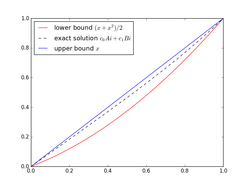
(xx2)/2 ≤ u(x) ≤ x

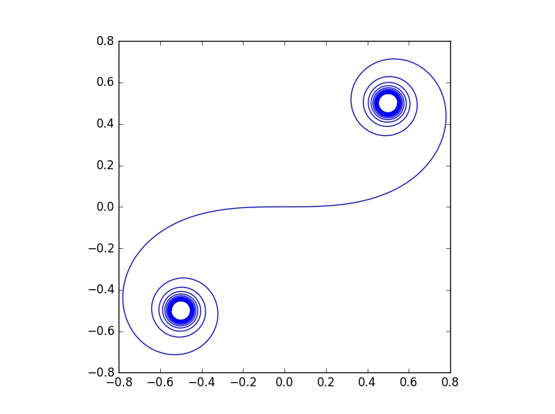
In general, you don’t know the function you’re trying to bound. That’s when bounds are most useful. But this is a sort of toy example because we do know the solution. The equation in this example is well known and is called Airy’s equation. The Airy functions Ai and Bi are independent solutions. Here’s a plot of the solution with its upper and lower bounds.

Here’s the Python code I used to solve for the coefficients of Ai and Bi and make the plot.

import numpy as np
from scipy.linalg import solve
from scipy.special import airy
import matplotlib.pyplot as plt

# airy(x) returns (Ai(x), Ai'(x), Bi(x), Bi'(x))
def Ai(x):
    return airy(x)[0]

def Bi(x):
    return airy(x)[2]

M = np.matrix([[Ai(0), Bi(0)], [Ai(1), Bi(1)]])
c = solve(M, [0, 1])

t = np.linspace(0, 1, 100)
plt.plot(t, (t + t**2)/2, 'r-', t, c[0]*Ai(t) + c[1]*Bi(t), 'k--', t, t, 'b-',)
plt.legend(["lower bound $(x + x^2)/2$", 
    "exact solution $c_0Ai + c_1Bi$", 
    "upper bound $x$"], loc="upper left")
plt.show()

SciPy’s function airy has an optimization that we waste here. The function computes Ai and Bi and their first derivatives all at the same time. We could take advantage of that to remove some redundant computations, but that would make the code harder to read. We chose instead to wait an extra nanosecond for the plot.

Help with differential equations

* * *

[1] Murray Protter and Hans Weinberger. Maximum Principles in Differential Equations.

Musical pitch notation

How can you convert the frequency of a sound to musical notation? I wrote in an earlier post how to calculate how many half steps a frequency is above or below middle C, but it would be useful go further have code to output musical pitch notation.

In scientific pitch notation, the C near the threshold of hearing, around 16 Hz, is called C0. The C an octave higher is C1, the next C2, etc. Octaves begin with C; other notes use the octave number of the closest C below.

C4, middle C

The lowest note on a piano is A0, a major sixth up from C0. Middle C is C4 because it’s 4 octaves above C0. The highest note on a piano is C8.

Math

A4, the A above middle C, has a frequency of 440 Hz. This is nine half steps above C4, so the pitch of C4 is 440*2−9/12. C0 is four octaves lower, so it’s 2−4 = 1/16 of the pitch of C4. (Details for this calculation and the one below are given in here.)

For a pitch P, the number of half steps from C0 to P is

h = 12 log2(P / C0).

Software

Here is a page that will let you convert back and forth between frequency and music notation: Music, Hertz, Barks.

If you’d like code rather than just to do one calculation, see the Python code below. It calculates the number of half steps h from C0 up to a pitch, then computes the corresponding pitch notation.

from math import log2, pow

A4 = 440
C0 = A4*pow(2, -4.75)
name = ["C", "C#", "D", "D#", "E", "F", "F#", "G", "G#", "A", "A#", "B"]
    
def pitch(freq):
    h = round(12*log2(freq/C0))
    octave = h // 12
    n = h % 12
    return name[n] + str(octave)

The pitch for A4 is its own variable in case you’d like to modify the code for a different tuning. While 440 is common, it used to be lower in the past, and you’ll sometimes see higher values like 444 today.

If you’d like to port this code to a language that doesn’t have a log2 function, you can use log(x)/log(2) for log2(x).

Powers of 2

When scientific pitch notation was first introduced, C0 was defined to be exactly 16 Hz, whereas now it works out to around 16.35. The advantage of the original system is that all C’s have frequency a power of 2, i.e. Cn has frequency 2n+4 Hz. The formula above for the number of half steps a pitch is above C0 simplifies to

h = 12 log2P − 48.

If C0 has frequency 16 Hz, the A above middle C has frequency 28.75 = 430.54, a little flat compared to A 440. But using the A 440 standard, C0 = 16 Hz is a convenient and fairly accurate approximation.

More posts on music and acoustics

General birthday problem

The birthday problem, sometimes called the birthday paradox, says that it’s more likely than you’d expect that two people in a group have the same birthday. Specifically, in a random sample of 23 people, there’s about a 50-50 chance that two people share the same birthday.

The birthday problem makes a nice party trick, but generalizations of the problem come up frequently in applications. I wrote in the previous post how it comes up in seeding distributed Monte Carlo simulations. In computer science, it’s a concern in hashing algorithms.

If you have a set of N things to choose from, such as N = 365 birthdays, and take r samples, the probability that all r samples are unique is

p = \frac{N!}{N^r (N-r)!}

and the probability that at least two of the samples are the same is 1 − p. (This assumes that N is at least as big as r. Otherwise the denominator is undefined, but in that case we know p is 0.)

With moderately large values of N and r the formula is likely to overflow if implemented directly. So as usual the trick is to use logarithms to avoid overflow or underflow. Here’s how you could compute the probability above in Python. SciPy doesn’t have a log factorial function, but does have a log gamma function, so we use that instead.

    from scipy import exp, log
    from scipy.special import gammaln

    def prob_unique(N, r):
        return exp( gammaln(N+1) - gammaln(N-r+1) - r*log(N) )


Related: Need help with randomization?

Spectral coordinates in Python

A graph doesn’t have any geometric structure unless we add it. The vertices don’t come with any position in space. The same graph can look very different when arranged different ways.

Spectral coordinates are a natural way to draw a graph because they are determined by the properties of the graph, not arbitrary aesthetic choices. Construct the Laplacian matrix and let x and y be the eigenvectors associated with the second and third eigenvalues. (The smallest eigenvalue is always zero and has an eigenvector of all 1’s. The second and third eigenvalues and eigenvectors are the first to contain information about a graph.) The spectral coordinates of the ith node are the ith components of x and y.

We illustrate this with a graph constructed from a dodecahedron, a regular solid with twenty vertices and twelve pentagonal faces. You can make a dodecahedron from a soccer ball by connecting the centers of all the white hexagons. Here’s one I made from Zometool pieces for a previous post:

Although we’re thinking of this graph as sitting in three dimensions, the nodes being the corners of pentagons etc., the graph simply says which vertices are connected to each other. But from this information, we can construct the graph Laplacian and use it to assign plane coordinates to each point. And fortunately, this produces a nice picture:

Here’s how that image was created using Python’s NetworkX library.

    import networkx as nx
    import matplotlib.pyplot as plt
    from scipy.linalg import eigh

    # Read in graph and compute the Laplacian L ...
    
    # Laplacian matrices are real and symmetric, so we can use eigh, 
    # the variation on eig specialized for Hermetian matrices.
    w, v = eigh(L) # w = eigenvalues, v = eigenvectors

    x = v[:,1] 
    y = v[:,2]
    spectral_coordinates = {i : (x[i], y[i]) for i in range(n)}
    G = nx.Graph()
    G.add_edges_from(graph)

    nx.draw(G, pos=spectral_coordinates)
    plt.show()

Update: After posting this I discovered that NetworkX has a method draw_spectral that will compute the spectral coordinates for you.

More spectral graph theory

Typesetting and computing continued fractions

Pi

The other day I ran across the following continued fraction for π.

\pi = 3 + \cfrac{1^2}{6+\cfrac{3^2}{6+\cfrac{5^2}{6+\cfrac{7^2}{6+\cdots}}}}

Source: L. J. Lange, An Elegant Continued Fraction for π, The American Mathematical Monthly, Vol. 106, No. 5 (May, 1999), pp. 456-458.

While the continued fraction itself is interesting, I thought I’d use this an example of how to typeset and compute continued fractions.

Typesetting

I imagine there are LaTeX packages that make typesetting continued fractions easier, but the following brute force code worked fine for me:

    \pi = 3 + \cfrac{1^2}{6+\cfrac{3^2}{6+\cfrac{5^2}{6+\cfrac{7^2}{6+\cdots}}}}

This relies on the amsmath package for the \cfrac command.

Computing

Continued fractions of the form

\pi = a_0 + \cfrac{b_1}{a_1+\cfrac{b_2}{a_2 +\cfrac{b_3}{a_3+\cfrac{b_4}{a_4+\cdots}}}}

can be computed via the following recurrence. Define A−1 = 1, A0 = a0, B−1 = 0, and B0 = 1. Then for k ≥ 1 define Ak+1 and Bk+1 by

A_{k+1} = a_{k+1}A_k + b_k A_{k-1} \\ B_{k+1} = a_{k+1}B_k + b_k B_{k-1}

Then the nth convergent the continued fraction is Cn = An / Bn.

The following Python code creates the a and b coefficients for the continued fraction for π above then uses a loop that could be used to evaluate any continued fraction.

    N = 20
    a = [3] + ([6]*N)
    b = [(2*k+1)**2 for k in range(0,N)]
    A = [0]*(N+1)
    B = [0]*(N+1)

    A[-1] = 1
    A[ 0] = a[0]
    B[-1] = 0
    B[ 0] = 1

    for n in range(1, N+1):
        A[n] = a[n]*A[n-1] + b[n-1]*A[n-2]
        B[n] = a[n]*B[n-1] + b[n-1]*B[n-2]
        print( n, A[n], B[n], A[n]/B[n] )

Python uses −1 as a shortcut to the last index of a list. I tack A−1 and B−1 on to the end of the A and B arrays to make the Python code match the math notation. This is either clever or a dirty hack, depending on your perspective.

Back to pi

You may notice that these approximations for π are not particularly good. It’s a trade-off for having a simple pattern to the coefficients. The continued fraction for π that has all b‘s equal to 1 has a complicated set of a‘s with no discernible pattern: 3, 7, 15, 1, 292, 1, 1, etc. However, that continued fraction produces very good approximations. If you replace the first three lines of the code above with that below, you’ll see that four iterations produces an approximation to π good to 10 decimal places.

    N = 4
    a = [3, 7, 15, 1, 292]
    b = [1]*N