Quantifying information gain in beta-binomial Bayesian model

Posted on 13 November 2017 by John

The beta-binomial model is the “hello world” example of Bayesian statistics. I would call it a toy model, except it is actually useful. It’s not nearly as complicated as most models used in application, but it illustrates the basics of Bayesian inference. Because it’s a conjugate model, the calculations work out trivially.

For more on the beta-binomial model itself, see A Bayesian view of Amazon Resellers and Functional Folds and Conjugate Models.

I mentioned in a recent post that the Kullback-Leibler divergence from the prior distribution to the posterior distribution is a measure of how much information was gained.

Here’s a little Python code for computing this. Enter the a and b parameters of the prior and the posterior to compute how much information was gained.

    from scipy.integrate import quad
    from scipy.stats import beta as beta
    from scipy import log2

    def infogain(post_a, post_b, prior_a, prior_b):

        p = beta(post_a, post_b).pdf
        q = beta(prior_a, prior_b).pdf

        (info, error) = quad(lambda x: p(x) * log2(p(x) / q(x)), 0, 1)
        return info

This code works well for medium-sized inputs. It has problems with large inputs because the generic integration routine quad needs some help when the beta distributions become more concentrated.

You can see that surprising input carries more information. For example, suppose your prior is beta(3, 7). This distribution has a mean of 0.3 and so your expecting more failures than successes. With such a prior, a success changes your mind more than a failure does. You can quantify this by running these two calculations.

    print( infogain(4, 7, 3, 7) )
    print( infogain(3, 8, 3, 7) )

The first line shows that a success would change your information by 0.1563 bits, while the second shows that a failure would change it by 0.0297 bits.

Why is Kullback-Leibler divergence not a distance?

Posted on 8 November 2017 by John

The Kullback-Leibler divergence between two probability distributions is a measure of how different the two distributions are. It is sometimes called a distance, but it’s not a distance in the usual sense because it’s not symmetric. At first this asymmetry may seem like a bug, but it’s a feature. We’ll explain why it’s useful to measure the difference between two probability distributions in an asymmetric way.

The Kullback-Leibler divergence between two random variables X and Y is defined as

$KL(X || Y) = -\int f_X(x) \log \frac{f_Y(x)}{f_X(x)} \, dx$

This is pronounced/interpreted several ways:

The divergence from Y to X
The relative entropy of X with respect to Y
How well Y approximates X
The information gain going from the prior Y to the posterior X
The average surprise in seeing Y when you expected X

A theorem of Gibbs proves that K-L divergence is non-negative. It’s clearly zero if X and Y have the same distribution.

The K-L divergence of two random variables is an expected value, and so it matters which distribution you’re taking the expectation with respect to. That’s why it’s asymmetric.

As an example, consider the probability densities below, one exponential and one gamma with a shape parameter of 2.

exponential and gamma PDFs

The two densities differ mostly on the left end. The exponential distribution believes this region is likely while the gamma does not. This means that an expectation with respect to the exponential distribution will weigh things in this region more heavily. In an information-theoretic sense, an exponential is a better approximation to a gamma than the other way around.

Here’s some Python code to compute the divergences.

    from scipy.integrate import quad
    from scipy.stats import expon, gamma
    from scipy import inf

    def KL(X, Y):
        f = lambda x: -X.pdf(x)*(Y.logpdf(x) - X.logpdf(x))
        return quad(f, 0, inf)

    e = expon
    g = gamma(a = 2)

    print( KL(e, g) )
    print( KL(g, e) )

This returns

    (0.5772156649008394, 1.3799968612282498e-08)
    (0.4227843350984687, 2.7366807708872898e-09)

The first element of each pair is the integral and the second is the error estimate. So apparently both integrals have been computed accurately, and the first is clearly larger. This backs up our expectation that it’s more surprising to see a gamma when expecting an exponential than vice versa.

Although K-L divergence is asymmetric in general, it can be symmetric. For example, suppose X and Y are normal random variables with the same variance but different means. Then it would be equally surprising to see either one when expecting the other. You can verify this in the code above by changing the KL function to integrate over the whole real line

    def KL(X, Y):
        f = lambda x: -X.pdf(x)*(Y.logpdf(x) - X.logpdf(x))
        return quad(f, -inf, inf)

and trying an example.

n1 = norm(1, 1)
n2 = norm(2, 1)

print( KL(n1, n2) )
print( KL(n2, n1) )

This returns

(0.4999999999999981, 1.2012834963423225e-08)
(0.5000000000000001, 8.106890774205374e-09)

and so both integrals are equal to within the error in the numerical integration.

Fourier-Bessel series and Gibbs phenomena

Posted on 4 November 2017 by John

Fourier-Bessel series are analogous to Fourier series. And like Fourier series, they converge pointwise near a discontinuity with the same kind of overshoot and undershoot known as the Gibbs phenomenon.

Fourier-Bessel series

Bessel functions come up naturally when working in polar coordinates, just as sines and cosines come up naturally when working in rectangular coordinates. You can think of Bessel functions as a sort of variation on sine waves. Or even more accurately, a variation on sinc functions, where sinc(z) = sin(z)/z. [1]

A Fourier series represents a function as a sum of sines and cosines of different frequencies. To make things a little simpler here, I’ll only consider Fourier sine series so I don’t have to repeatedly say “and cosine.”

$f(z) = \sum_{n=1}^\infty c_n \sin(n \pi z)$

A Fourier-Bessel function does something similar. It represents a function as a sum of rescaled versions of a particular Bessel function. We’ll use the Bessel J₀ here, but you could pick some other J_ν.

Fourier series scale the sine and cosine functions by π times integers, i.e. sin(πz), sin(2πz), sin(3πz), etc. Fourier-Bessel series scale by the zeros of the Bessel function: J₀(λ₁z), J₀(λ₂z), J₀(λ₃z), etc. where λ_n are the zeros of J₀. This is analogous to scaling sin(πz) by its roots: π, 2π, 3π, etc. So a Fourier-Bessel series for a function f looks like

$f(z) = \sum_{n=1}^\infty c_n J_0(\lambda_n z).$

The coefficients c_n for Fourier-Bessel series can be computed analogously to Fourier coefficients, but with a couple minor complications. First, the basis functions of a Fourier series are orthogonal over [0, 1] without any explicit weight, i.e. with weight 1. And second, the inner product of a basis function doesn’t depend on the frequency. In detail,

$\int_0^1 \sin(m \pi z) \, \sin(n \pi z) \, dz = \frac{\delta_{mn}}{2}.$

Here δ_mn equals 1 if m = n and 0 otherwise.

Fourier-Bessel basis functions are orthogonal with a weight z, and the inner product of a basis function with itself depends on the frequency. In detail

$\int_0^1 J_0(\lambda_m z) \, J_0(\lambda_n z) \, z\, dz = \frac{\delta_{mn}}{2} J_1(\lambda_n).$

So whereas the coefficients for a Fourier sine series are given by

$c_n = 2 \int_0^1 f(z)\, \sin(n\pi z) \,dz$

the coefficients for a Fourier-Bessel series are given by

$c_n = \frac{ 2\int_0^1 f(z)\, J_0(\lambda_n z) \, dz}{ J_1(\lambda_n)^2 }.$

Gibbs phenomenon

Fourier and Fourier-Bessel series are examples of orthogonal series, and so by construction they converge in the norm given by their associated inner product. That means that if S_N is the Nth partial sum of a Fourier series

$\lim_{N\to\infty} \int_0^1 \left( f(x) - S_N(x) \right)^2 \, dz = 0$
and the analogous statement for a Fourier-Bessel series is

$\lim_{N\to\infty} \int_0^1 \left( f(x) - S_N(x) \right)^2 \, z\, dz = 0.$

In short, the series converge in a (weighted) L² norm. But how do the series converge pointwise? A lot of harmonic analysis is devoted to answering this question, what conditions on the function f guarantee what kind of behavior of the partial sums of the series expansion.

If we look at the Fourier series for a step function, the partial sums converge pointwise everywhere except at the step discontinuity. But the way they converge is interesting. You get a sort of “bat ear” phenomena where the partial sums overshoot the step function at the discontinuity. This is called the Gibbs phenomenon after Josiah Willard Gibbs who observed the effect in 1899. (Henry Wilbraham observed the same thing earlier, but Gibbs didn’t know that.)

The Gibbs phenomena is well known for Fourier series. It’s not as well known that the same phenomenon occurs for other orthogonal series, such as Fourier-Bessel series. I’ll give an example of Gibbs phenomenon for Fourier-Bessel series taken from [2] and give Python code to visualize it.

We take our function f(z) to be 1 on [0, 1/2] and 0 on (1/2, 1]. It works out that

$c_n = \frac{1}{\lambda_n} \frac{J_1(\lambda_n / 2)}{ J_1(\lambda_n)^2 }.$

Python code and plot

Here’s the plot with 100 terms. Notice how the partial sums overshoot the mark to the left of 1/2 and undershoot to the right of 1/2.

Plot showing Gibbs phenomena for Fourier-Bessel series

Here’s the same plot with 1,000 terms.

Gibbs phenomena for 1000 terms of Fourier-Bessel series

Here’s the Python code that produced the plot.

    import matplotlib.pyplot as plt
    from scipy.special import j0, j1, jn_zeros
    from scipy import linspace

    N = 100 # number of terms in series

    roots = jn_zeros(0, N)
    coeff = [j1(r/2) / (r*j1(r)**2) for r in roots]
    z = linspace(0, 1, 200)

    def partial_sum(z):
        return sum( coeff[i]*j0(roots[i]*z) for i in range(N) )

    plt.plot(z, partial_sum(z))
    plt.xlabel("z")
    plt.ylabel("{}th partial sum".format(N))
    plt.show()

Footnotes

[1] To be precise, as z goes to infinity

$J_nu(z) sim sqrt{frac{2}{pi z}} cosleft(z - frac{1}{2} nu pi - frac{pi}{4} right)$

and so the Bessel functions are asymptotically proportional to sin(z – φ)/√z for some phase shift φ.

[2] The Gibbs’ phenomenon for Fourier-Bessel Series. Temple H. Fay and P. Kendrik Kloppers. International Journal of Mathematical Education in Science and Technology. 2003. vol. 323, no. 2, 199-217.

Approximate inverse of the gamma function

Posted on 11 February 2017 by John

The other day I ran across a blog post by Brian Hayes that linked to an article by David Cantrell on how to compute the inverse of the gamma function. Cantrell gives an approximation in terms of the Lambert W function.

In this post we’ll write a little Python code to kick the tires on Cantrell’s approximation. The post also illustrates how to do some common tasks using SciPy and matplotlib.

Here are the imports we’ll need.

      import matplotlib.pyplot as plt
      from scipy import pi, e, sqrt, log, linspace
      from scipy.special import lambertw, gamma, psi
      from scipy.optimize import root

First of all, the gamma function has a local minimum k somewhere between 1 and 2, and so it only makes sense to speak of its inverse to the left or right of this point. Gamma is strictly increasing for real values larger than k.

To find k we look for where the derivative of gamma is zero. It’s more common to work with the derivative of the logarithm of the gamma function than the derivative of the gamma function itself. That works just as well because gamma has a minimum where its log has a minimum. The derivative of the log of the gamma function is called ψ and is implemented in SciPy as scipy.special.psi. We use the function scipy.optimize.root to find where ψ is zero.

The root function returns more information than just the root we’re after. The root(s) are returned in the arrayx, and in our case there’s only one root, so we take the first element of the array:

      k = root(psi, 1.46).x[0]

Now here is Cantrell’s algorithm:

      c = sqrt(2*pi)/e - gamma(k)
      
      def L(x):
          return log((x+c)/sqrt(2*pi))
      
      def W(x):
          return lambertw(x)
      
      def AIG(x):
          return L(x) / W( L(x) / e) + 0.5

Cantrell uses AIG for Approximate Inverse Gamma.

How well goes this algorithm work? For starters, we’ll see how well it does when we do a round trip, following the exact gamma with the approximate inverse.

      x = linspace(5, 30, 100)
      plt.plot(x, AIG(gamma(x)))
      plt.show()

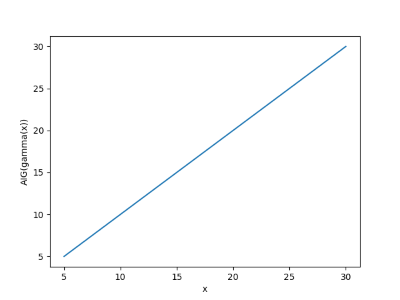
This produces the following plot:

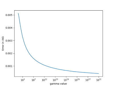
We get a straight line, as we should, so next we do a more demanding test. We’ll look at the absolute error in the approximate inverse. We’ll use a log scale on the x-axis since gamma values get large quickly.

      y = gamma(x)
      plt.plot(y, x- AIG(y))
      plt.xscale("log")
      plt.show()

This shows the approximation error is small, and gets smaller as its argument increases.

Cantrell’s algorithm is based on an asymptotic approximation, so it’s not surprising that it improves for large arguments.

Random squares

Posted on 8 November 2016 by John

In geometry, you’d say that if a square has side x, then it has area x².

In calculus, you’d say more. First you’d say that if a square has side near x, then it has area near x². That is, area is a continuous function of the length of a side. As the length of the side changes, there’s never an abrupt jump in area. Next you could be more specific and say that a small change Δx to a side of length x corresponds to approximately a change of 2x Δx in the area.

In probability, you ask what is the area of a square like if you pick the length of its side at random. If you pick the length of the side from a distribution with mean μ, does the distribution of the area have mean μ²? No, but if the probability distribution on side length is tightly concentrated around μ, then the distribution on area will be concentrated near μ². And you can approximate just how near the area is to μ² using the delta method, analogous to the calculus discussion above.

If the distribution on side lengths is not particularly concentrated, finding the distribution on the area is more interesting. It will depend on the specific distribution on side length, and the mean area might not be particularly close to the square of the mean side length. The function to compute area is trivial, and yet the question of what happens when you stick a random variable into that function is not trivial. Random variables behave as you might expect when you stick them into linear functions, but offer surprises when you stick them into nonlinear functions.

Suppose you pick the length of the side of a square uniformly from the interval [0, 1]. Then the average side is 1/2, and so you might expect the average area to be 1/4. But the expected area is actually 1/3. You could see this a couple ways, analytically and empirically.

First an analytical derivation. If X has a uniform [0, 1] distribution and Z = X², then the CDF of Z is

Prob(Z ≤ z) = Prob(X ≤ √z) = √ z.

and so the PDF for Z, the derivative of the CDF, is -1/2√z. From there you can compute the expected value by integrating z times the PDF.

You could check your calculations by seeing whether simulation gives you similar results. Here’s a little Python code to do that.

      from random import random
      N = 1000000
      print( sum( random()**2 for _ in range(N) )/N )

When I run this, I get 0.33386, close to 1/3.

Now lets look at an exponential distribution on side length with mean 1. Then a calculation similar to the one above shows that the expected value of the product is 2. You can also check this with simulation. This time we’ll be a little fancier and let SciPy generate our random values for us.

      print( sum(expon.rvs(size=N)**2)/N )

When I ran this, I got 1.99934, close to the expected value of 2.

You’ll notice that in both examples, the expected value of the area is more than the square of the expected value of the side. This is not a coincidence but consequence of Jensen’s inequality. Squaring is a convex function, so the expected value of the square is larger than the square of the expected value for any random variable.

Distribution of numbers in Pascal’s triangle

Posted on 5 July 2016 by John

This post explores a sentence from the book Single Digits:

Any number in Pascal’s triangle that is not in the outer two layers will appear at least three times, usually four.

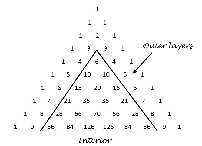
Pascal’s triangle contains the binomial coefficients C(n, r) where n ranges over non-negative numbers and r ranges from 0 to n. The outer layers are the elements with r equal to 0, 1, n-1, and n.

Pascal's triangle

We’ll write some Python code to explore how often the numbers up to 1,000,000 appear. How many rows of Pascal’s triangle should we compute? The smallest number on row n is C(n, 2). Now 1,000,000 is between C(1414, 2) and C(1415, 2) so we need row 1414. This means we need N = 1415 below because the row numbers start with 0.

I’d like to use a NumPy array for storing Pascal’s triangle. In the process of writing this code I realized that a NumPy array with dtype int doesn’t contain Python’s arbitrary-sized integers. This makes sense because NumPy is designed for efficient computation, and using a NumPy array to contain huge integers is unnatural. But I’d like to do it anyway, and the way to make it happen is to set dtype to object.

    import numpy as np
    from collections import Counter
    
    N = 1415 # Number of rows of Pascal's triangle to compute
    
    Pascal = np.zeros((N, N), dtype=object)
    Pascal[0, 0] = 1
    Pascal[1,0] = Pascal[1,1] = 1
    
    for n in range(2, N):
        for r in range(0, n+1):
            Pascal[n, r] = Pascal[n-1, r-1] + Pascal[n-1, r]
    
    c = Counter()
    for n in range(4, N):
        for r in range(2, n-1):
            p = Pascal[n, r]
            if p <= 1000000:
                c[p] += 1

When we run this code, we find that our counter contains 1732 elements. That is, of the numbers up to one million, only 1732 of them appear inside Pascal’s triangle when we disallow the outer two layers. (The second layer contains consecutive integers, so every positive integer appears in Pascal’s triangle. But most integers only appear in the second layer.)

When Single Digits speaks of “Any number in Pascal’s triangle that is not in the outer two layers” this cannot refer to numbers that are not in the outer two layers because every natural number appears in the outer two layers. Also, when it says the number “will appear at least three times, usually four” it is referring to the entire triangle, i.e. including the outer two layers. So another way to state the sentence quoted above is as follows.

Define the interior of Pascal’s triangle to be the triangle excluding the outer two layers. Every number n in the interior of Pascal’s triangle appears twice more outside of the interior, namely as C(n, 1) and C(n, n-1). Most often n appears at least twice in the interior as well.

This means that any number you find in the interior of Pascal’s triangle, interior meaning not in the two outer layers, will appear at least three times in the full triangle, usually more.

Here are the statistics from our code above regarding just the interior of Pascal’s triangle.

One number, 3003, appears six times.
Six numbers appear four times: 120, 210, 1540, 7140, 11628, and 24310.
Ten numbers appear only once: 6, 20, 70, 252, 924, 3432, 12870, 48620, 184756, and 705432.
The large majority of numbers, 1715 out of 1732, appear twice.

How to create Green noise in Python

Posted on 27 April 2016 by John

This is a follow-on to my previous post on green noise. Here we create green noise with Python by passing white noise through a Butterworth filter.

Green noise is in the middle of the audible spectrum (on the Bark scale), just where our hearing is most sensitive, analogous to the green light, the frequency where our eyes are most sensitive. See previous post for details, including an explanation of where the left and right cutoffs below come from.

Here’s the code:

from scipy.io.wavfile import write
from scipy.signal import buttord, butter, filtfilt
from scipy.stats import norm
from numpy import int16

def turn_green(signal, samp_rate):
    # start and stop of green noise range
    left = 1612 # Hz
    right = 2919 # Hz

    nyquist = (samp_rate/2)
    left_pass  = 1.1*left/nyquist
    left_stop  = 0.9*left/nyquist
    right_pass = 0.9*right/nyquist
    right_stop = 1.1*right/nyquist

    (N, Wn) = buttord(wp=[left_pass, right_pass],
                      ws=[left_stop, right_stop],
                      gpass=2, gstop=30, analog=0)
    (b, a) = butter(N, Wn, btype='band', analog=0, output='ba')
    return filtfilt(b, a, signal)

def to_integer(signal):
    # Take samples in [-1, 1] and scale to 16-bit integers,
    # values between -2^15 and 2^15 - 1.
    signal /= max(signal)
    return int16(signal*(2**15 - 1))

N = 48000 # samples per second

white_noise= norm.rvs(0, 1, 3*N) # three seconds of audio
green = turn_green(white_noise, N)
write("green_noise.wav", N, to_integer(green))

And here’s what it sounds like:

(download .wav file)

Let’s look at the spectrum to see whether it looks right. We’ll use one second of the signal so the x-axis coincides with frequency when we plot the FFT.

from scipy.fftpack import fft

one_sec = green[0:N]
plt.plot(abs(fft(one_sec)))
plt.xlim((1500, 3000))
plt.show()

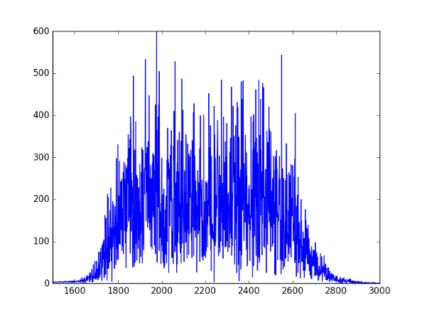
Here’s the output, concentrated between 1600 and 3000 Hz as expected:

spectral plot of green noise

Creating police siren sounds with frequency modulation

Posted on 10 March 2016 by John

Yesterday I was looking into calculating fluctuation strength and playing around with some examples. Along the way I discovered how to create files that sound like police sirens. These are sounds with high fluctuation strength.

police car lights

The Python code below starts with a carrier wave at f_c = 1500 Hz. Not surprisingly, this frequency is near where hearing is most sensitive. Then this signal is modulated with a signal with frequency f_m. This frequency determines the frequency of the fluctuations.

The slower example produced by the code below sounds like a police siren. The faster example makes me think more of an ambulance or fire truck. Next time I hear an emergency vehicle I’ll pay more attention.

If you use a larger value of the modulation index β and a smaller value of the modulation frequency f_m you can make a sound like someone tuning a radio, which is no coincidence.

Here are the output audio files in .wav format:

slow.wav

fast.wav

from scipy.io.wavfile import write
from numpy import arange, pi, sin, int16

def f(t, f_c, f_m, beta):
    # t    = time
    # f_c  = carrier frequency
    # f_m  = modulation frequency
    # beta = modulation index
    return sin(2*pi*f_c*t - beta*sin(2*f_m*pi*t))

def to_integer(signal):
    # Take samples in [-1, 1] and scale to 16-bit integers,
    # values between -2^15 and 2^15 - 1.
    return int16(signal*(2**15 - 1))

N = 48000 # samples per second
x = arange(3*N) # three seconds of audio

data = f(x/N, 1500, 2, 100)
write("slow.wav", N, to_integer(data))

data = f(x/N, 1500, 8, 100)
write("fast.wav", N, to_integer(data))

Maximum principle and approximating boundary value problems

Posted on 10 February 2016 by John

Solutions to differential equations often satisfy some sort of maximum principle, which can in turn be used to construct upper and lower bounds on solutions.

We illustrate this in one dimension, using a boundary value problem for an ordinary differential equation (ODE).

Maximum principles

If the second derivative of a function is positive over an open interval (a, b), the function cannot have a maximum in that interval. If the function has a maximum over the closed interval [a, b] then it must occur at one of the ends, at a or b.

This can be generalized, for example, to the following maximum principle. Let L be the differential operator

L[u] = u” + g(x)u’ + h(x)

where g and h are bounded functions on some interval [a, b] and h is non-positive. Suppose L[u] ≥ 0 on (a, b). If u has an interior maximum, then u must be constant.

Boundary value problems

Now suppose that we’re interested in the boundary value problem L[u] = f where we specify the values of u at the endpoints a and b, i.e. u(a) = u_a and u(b) = u_b. We can construct an upper bound on u as follows.

Suppose we find a function z such that L[z] ≤ f and z(a) ≥ u_a and z(b) ≥ u_b. Then by applying the maximum principle to u – z, we see that u – z must be ≤ 0, and so z is an upper bound for u.

Similarly, suppose we find a function w such that L[w] ≥ f and w(a) ≤ u_a and w(b) ≤ u_b. Then by applying the maximum principle to w – u, we see that w – u must be ≤ 0, and so w is an lower bound for u.

Note that any functions z and w that satisfy the above requirements give upper and lower bounds, though the bounds may not be very useful. By being clever in our choice of z and w we may be able to get tighter bounds. We might start by choosing polynomials, exponentials, etc. Any functions that are easy to work with and see how good the resulting bounds are.

Tomorrow’s post is similar to this one but looks at bounds for an initial value problem rather than a boundary value problem.

Airy equation example

The following is an elaboration on an example from [1]. Suppose we want to bound solutions to

u”(x) – x u(x) = 0

where u(0) = 0 and u(1) = 1. (This is a well-known equation, but for purposes of illustration we’ll pretend at first that we know nothing about its solutions.)

For our upper bound, we can simply use z(x) = x. We have L[z] ≤ 0 and z satisfies the boundary conditions exactly.

For our lower bound, we use w(x) = x – βx(1 – x). Why? The function z already satisfies the boundary condition. If we add some multiple of x(1 – x) we’ll maintain the boundary condition since x(1 – x) is zero at 0 and 1. The coefficient β gives us some room to maneuver. Turns out L[w] ≥ 0 if β ≥ 1/2. If we choose β = 1/2 we have

(x + x²)/2 ≤ u(x) ≤ x

In general, you don’t know the function you’re trying to bound. That’s when bounds are most useful. But this is a sort of toy example because we do know the solution. The equation in this example is well known and is called Airy’s equation. The Airy functions Ai and Bi are independent solutions. Here’s a plot of the solution with its upper and lower bounds.

Here’s the Python code I used to solve for the coefficients of Ai and Bi and make the plot.

import numpy as np
from scipy.linalg import solve
from scipy.special import airy
import matplotlib.pyplot as plt

# airy(x) returns (Ai(x), Ai'(x), Bi(x), Bi'(x))
def Ai(x):
    return airy(x)[0]

def Bi(x):
    return airy(x)[2]

M = np.matrix([[Ai(0), Bi(0)], [Ai(1), Bi(1)]])
c = solve(M, [0, 1])

t = np.linspace(0, 1, 100)
plt.plot(t, (t + t**2)/2, 'r-', t, c[0]*Ai(t) + c[1]*Bi(t), 'k--', t, t, 'b-',)
plt.legend(["lower bound $(x + x^2)/2$", 
    "exact solution $c_0Ai + c_1Bi$", 
    "upper bound $x$"], loc="upper left")
plt.show()

SciPy’s function airy has an optimization that we waste here. The function computes Ai and Bi and their first derivatives all at the same time. We could take advantage of that to remove some redundant computations, but that would make the code harder to read. We chose instead to wait an extra nanosecond for the plot.

Help with differential equations

* * *

[1] Murray Protter and Hans Weinberger. Maximum Principles in Differential Equations.

Dilogarithm, polylogarithm, and related functions

Posted on 5 February 2016 by John

The functions dilogarithm, trilogarithm, and more generally polylogarithm are meant to be generalizations of the logarithm. I first came across the dilogarithm in college when I was evaluating some integral with Mathematica, and they’ve paid a visit occasionally ever since.

Unfortunately polylogarithms are defined in several slightly different and incompatible ways. I’ll start by following An Atlas of Functions and then mention differences in A&S, SciPy, and Mathematica.

Polylogarithms

According to Atlas,

Polylogarithms are themselves special cases of Lerch’s function. Also known as Jonquière’s functions (Ernest Jean Philippe Fauque de Jonquières, 1820–1901, French naval officer and mathematician), they appear in the Feynman diagrams of particle physics.

The idea is to introduce an extra parameter ν in the power series for natural log:

$\mbox{polyln}_\nu(x) = -\sum_{j=1}^\infty \frac{(1-x)^j}{j^\nu}$

When ν = 1 we get the ordinary logarithm, i.e. polyln₁ = log. Then polyln₂ is the dilogarithm diln, and polyln₃ is the trilogarithm triln.

One advantage of the definition in Atlas is that the logarithm is a special case of the polylogarithm. Other conventions don’t have this property.

Other conventions

The venerable A&S defines dilogarithms in a way that’s equivalent to the negative of the definition above and does not define polylogarithms of any other order. SciPy’s special function library follows A&S. SciPy uses the name spence for the dilogarithm for reasons we’ll get to shortly.

Mathematica has the function PolyLog[ν, x] that evaluates to

$\mbox{Li}_\nu(x) = \sum_{j=1}^\infty \frac{x^j}{j^\nu}$

So polyln_ν above corresponds to -PolyLog[ν, -x] in Mathematica. Matlab’s polylog is the same as Mathematica’s PolyLog.

Relation to other functions

Spence’s integral is the function of x given by the integral

$\int_1^x \frac{\log t}{t-1}\, dt$

and equals diln(x). Note that the SciPy function spence returns the negative of the integral above.

The Lerch function mentioned above is named for Mathias Lerch (1860–1922) and is defined by the integral

$\Phi(x, \nu, u) = \frac{1}{\Gamma(\nu)} \int_0^\infty \frac{t^{\nu-1} \exp(-ut)}{1 - x\exp(-t)} \, dt$

The connection with polylogarithms is easier to see from the series expansion:

$\Phi(x, \nu, u) = \sum_{j=0}^\infty \frac{x^j}{(j+u)^\nu}$

The connection with polylogarithms is then

$\Phi(x, \nu,1) = -\frac{1}{x} \mbox{polyln}_\nu(1-x)$

Note that the Lerch function also generalizes the Hurwitz zeta function, which in turn generalizes the Riemann zeta function. When x = 1, the Lerch function reduces to ζ(ν, u).

Related: Applied complex analysis

SciPy