Pareto and Pandas

This post muses about what it means to learn a software library. I’ll use Pandas as an example, but the post isn’t just about Pandas.

Suppose you say “I want to learn Pandas.” That implicitly assumes Pandas one thing, and in a sense it is. In another sense Pandas is hundreds of things.

At the top level, the pandas module (version 1.2.0) has 142 things inside.

    >>> import pandas as pd
    >>> len(dir(pd))
    142

The two most important things inside are the Series and DataFrame objects. They each in turn contain hundreds of things.

    >>> len(dir(pd.Series))
    434
    >>> len(dir(pd.DataFrame))
    441

That’s evidence Pandas’ diversity. But here’s evidence of it’s unity: most of the things inside these two objects have the same names.

    >>> s = set(dir(pd.Series))
    >>> d = set(dir(pd.DataFrame))
    >>> len(s.union(d))
    491
    >>> len(s - d)
    50
    >>> len(d - s)
    57

Pandas kinda has a fractal dimension, having both complexity and unity. The best way to think about it is not as one monolithic thing, or as hundreds of isolated things. It’s a coherent, but not perfectly coherent, collection of related things. This is true of all software libraries. Pandas is more coherent than most libraries because it was initially the product of one mind, that of Wes McKinney.

This has a couple implications for what it means to “learn Pandas.” Because Pandas is big, you have to explore it strategically, not exhaustively. And because Pandas is coherent, part of what it means to learn Pandas is to develop a feel for the way Pandas does things.

No one is going to learn Pandas by studying every object, every method on every object, and every argument to every method on every object. It’s too big. That’s also unnecessary.

There’s probably something like a Pareto distribution on the usefulness of features. The most commonly used features are used far, far more often than the most obscure features.

It would be interesting to do some kind of survey to see which features are actually used and how often. But I don’t think that’s practical. The easiest thing to do would be to find some large code base that heavily uses Pandas. But that’s not typical of how Pandas is used. Probably most lines of code using Pandas are scattered over millions of small scripts, much of it not in production code.

A well-designed library makes it possible to make good guesses about functionality you haven’t used. You learn the gestalt of the library. You can always look up API documentation as needed, but you can’t develop an intuition for a library just-in-time.

“Learn Pandas” is a daunting goal, and maybe an impossible goal if by “learn” you mean explore exhaustively. But “learn how to do my common tasks quickly in Pandas” and “develop a feel for how to do things in Pandas” are much smaller tasks.

Related posts

Broadcasting and functors

In my previous post, I looked at the map Δ that takes a column vector to a diagonal matrix. I even drew a commutative diagram, which foreshadows a little category theory.

Suppose you have a function f of a real or complex variable. To an R programmer, if x is a vector, it’s obvious that f(x) means to apply f to every component of a vector. Python (NumPy) works the same way, and calls this broadcasting. To a mathematician, this looks odd. What does the logarithm of a vector, for example, even mean?

As in the previous post, we can use Δ to formalize things. We said that Δ has some nice properties, and in fact we will show it is a functor.

To have a functor, we have to have categories. (Historically, functors came first; categories were defined in order to define functors.) We will define C to be the category of column vectors and M the category of square matrices as before. Or rather, we should say the objects of C are column vectors and the objects of M are square matrices.

Categories need morphisms, functions between objects [1]. We define the morphisms on C to be analytic functions applied componentwise. So, for example, if

z = [1, 2, -3],

then

tan(z) = [tan(1), tan(2), tan(-3)].

The morphisms on M will be analytic functions on square matrices, not applied componentwise but applied by power series. That is, given an analytic function f, we define f of a square matrix X as the result of sticking the matrix X into the power series for f. For an example, see What is the cosine of a matrix?

We said that Δ is a functor. It takes column vectors and turns them into square matrices by putting their contents along the diagonal of a matrix. We gave the example in the previous post that [4, i, π] would be mapped to the matrix with these elements on the diagonal, i.e.

\Delta: \begin{pmatrix} 4 \\ i \\ \pi \end{pmatrix} \mapsto \begin{pmatrix} 4 & 0 & 0\\ 0 & i & 0 \\ 0 & 0 & \pi \end{pmatrix}

That says what Δ does on objects, but what does it do on morphisms? It takes an analytic function that was applied componentwise to column vectors, and turns it into a function that is applied via its power series to square matrices. That is, starting with a function

f(z) = \sum_{n=0}^\infty a_nz^n

we define the morphism f on C by

f : \begin{pmatrix} z_1 \\ z_2 \\ \vdots \\ z_n \end{pmatrix} \mapsto \begin{pmatrix} f(z_1) \\ f(z_2) \\ \vdots \\ f(z_n) \end{pmatrix}

and the morphism Δ f on M by

\Delta f : Z \mapsto \sum_{n=0}^\infty a_n Z^n

where Z is a square matrix.

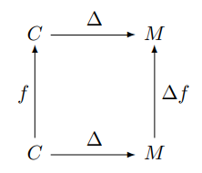
We can apply f to a column vector, and then apply Δ to turn the resulting vector into a diagonal matrix, or we could apply Δ to turn the vector into a diagonal matrix first, and then apply f (technically,  Δf). That is, the follow diagram commutes:

\begin{diagram}   C & \rTo^{\Delta} & M \\   \uTo^{f} & & \uTo_{\Delta f} \\   C & \rTo^{\Delta} & M  \end{diagram}

Python example

Applying an analytic function to a diagonal matrix gives the same result as simply applying the function to the elements of the diagonal. But for more general square matrices, this is not the case. We will illustrate this with some Python code.

    import numpy as np
    from scipy.linalg import funm

    d = np.array([1, 2])
    D = np.diag(d)
    M = np.array([[1, np.pi], [2, 0]])

Now let’s look at some output.

    >>> np.sin(d)                     
    array([0.84147098, 0.90929743])   

    >>> np.sin(D)                     
    array([[0.84147098, 0.        ],  
           [0.        , 0.90929743]]) 

    >>> funm(D, np.sin)               
    array([[0.84147098, 0.        ],  
           [0.        , 0.90929743]]) 

So if we take the sine of d and turn the result into a matrix, we get the same thing as if we turn d into a matrix D and then take the sine of D, either componentwise or as an analytic function (with funm, function of a matrix).

Now let’s look at a general, non-diagonal matrix.

    >>> np.sin(M)
    array([[0.84147099, 0],
       [0.90929743, 0]])

    >>> funm(D, np.sin)
    array([[0.84147098, 0.        ],
           [0.        , 0.90929743]])

Note that the elements in the bottom row are in opposite positions in the two examples.

[1] OK, morphisms are not necessarily functions, but in practice they usually are.

Python triple quote strings and regular expressions

There are several ways to quote strings in Python. Triple quotes let strings span multiple lines. Line breaks in your source file become line break characters in your string. A triple-quoted string in Python acts something like “here doc” in other languages.

However, Python’s indentation rules complicate matters because the indentation becomes part of the quoted string. For example, suppose you have the following code outside of a function.

x = """\
abc
def
ghi
"""

Then you move this into a function foo and change its name to y.

def foo():
    y = """\
    abc
    def
    ghi
    """

Now x and y are different strings! The former begins with a and the latter begins with four spaces. (The backslash after the opening triple quote prevents the following newline from being part of the quoted string. Otherwise x and y would begin with a newline.) The string y also has four spaces in front of def and four spaces in front of ghi. You can’t push the string contents to the left margin because that would violate Python’s formatting rules. (Update: Oh yes you can! See Aaron Meurer’s comment below.)

We now give three solutions to this problem.

Solution 1: textwrap.dedent

There is a function in the Python standard library that will strip the unwanted space out of the string y.

import textwrap 

def foo():
    y = """\
    abc
    def
    ghi
    """
    y = textwrap.dedent(y)

This works, but in my opinion a better approach is to use regular expressions [1].

Solution 2: Regular expression with a flag

We want to remove white space, and the regular expression for a white space character is \s. We want to remove one or more white spaces so we add a + on the end. But in general we don’t want to remove all white space, just white space at the beginning of a line, so we stick ^ on the front to say we want to match white space at the beginning of a line.

import re 

def foo():
    y = """\
    abc
    def
    ghi
    """
    y = re.sub("^\s+", "", y)

Unfortunately this doesn’t work. By default ^ only matches the beginning of a string, not the beginning of a line. So it will only remove the white space in front of the first line; there will still be white space in front of the following lines.

One solution is to add the flag re.MULTILINE to the substitution function. This will signal that we want ^ to match the beginning of every line in our multi-line string.

    y = re.sub("^\s+", "", y, re.MULTILINE)

Unfortunately that doesn’t quite work either! The fourth positional argument to re.sub is a count of how many substitutions to make. It defaults to 0, which actually means infinity, i.e. replace all occurrences. You could set count to 1 to replace only the first occurrence, for example. If we’re not going to specify count we have to set flags by name rather than by position, i.e. the line above should be

    y = re.sub("^\s+", "", y, flags=re.MULTILINE)

That works.

You could also abbreviate re.MULTILINE to re.M. The former is more explicit and the latter is more compact. To each his own. There’s more than one way to do it. [2]

Solution 3: Regular expression with a modifier

In my opinion, it is better to modify the regular expression itself than to pass in a flag. The modifier (?m) specifies that in the rest of the regular the ^ character should match the beginning of each line.

    y = re.sub("(?m)^\s+", "", y)

One reason I believe this is better is that moves information from a language-specific implementation of regular expressions into a regular expression syntax that is supported in many programming languages.

For example, the regular expression

    (?m)^\s+

would have the same meaning in Perl and Python. The two languages have the same way of expressing modifiers [3], but different ways of expressing flags. In Perl you paste an m on the end of a match operator to accomplish what Python does with setting flasgs=re.MULTILINE.

One of the most commonly used modifiers is (?i) to indicate that a regular expression should match in a case-insensitive manner. Perl and Python (and other languages) accept (?i) in a regular expression, but each language has its own way of adding modifiers. Perl adds an i after the match operator, and Python uses

    flags=re.IGNORECASE

or

    flags=re.I

as a function argument.

More on regular expressions

[1] Yes, I’ve heard the quip about two problems. It’s funny, but it’s not a universal law.

[2] “There’s more than one way to do it” is a mantra of Perl and contradicts The Zen of Python. I use the line here as a good-natured jab at Python. Despite its stated ideals, Python has more in common with Perl than it would like to admit and continues to adopt ideas from Perl.

[3] Python’s re module doesn’t support every regular expression modifier that Perl supports. I don’t know about Python’s regex module.

Searching Greek and Hebrew with regular expressions

According to the Python Cookbook, “Mixing Unicode and regular expressions is often a good way to make your head explode.” It is thus with fear and trembling that I dip my toe into using Unicode with Greek and Hebrew.

I heard recently that there are anomalies in the Hebrew Bible where the final form of a letter is deliberately used in the middle of a word. That made me think about searching for such anomalies with regular expressions. I’ll come back to that shortly, but I’ll start by looking at Greek where things are a little simpler.

Greek

Only one letter in Greek has a variant form at the end of a word. Sigma is written ς at the end of a word and σ everywhere else. The following Python code shows we can search for sigmas and final sigmas in the first sentence from Matthew’s gospel.

    import re

    matthew = "Κατάλογος του γένους του Ιησού Χριστού, γιου του Δαυείδ, γιου του Αβραάμ"
    matches = re.findall(r"\w+ς\b", matthew)
    print("Words ending in sigma:", matches)

    matches = re.findall(r"\w*σ\w+", matthew)
    print("Words with non-final sigmas:", matches)

This prints

    Words ending in sigma: ['Κατάλογος', 'γένους']
    Words with non-final sigmas: ['Ιησού', 'Χριστού']

This shows that we can use non-ASCII characters in regular expressions, at least if they’re Greek letters, and that the metacharacters \w (word character) and \b (word boundary) work as we would hope.

Hebrew

Now for the motivating example. Isaiah 9:6 contains the word “לםרבה” with the second letter (second from right) being the final form of Mem, ם, sometimes called “closed Mem” because the form of the letter ordinarily used in the middle of a word, מ, is not a closed curve [1].

Here’s code to show we could find this anomaly with regular expressions.

    # There are five Hebrew letters with special final forms.
    finalforms = "\u05da\u05dd\u05df\u05e3\u05e5" # ךםןףץ

    lemarbeh = "\u05dc\u05dd\u05e8\u05d1\u05d4" # לםרבה
    m = re.search(r"\w*[" + finalforms + "\w+", lemarbeh)
    if m:
        print("Anomaly found:", m.group(0))

As far as I know, the instance discussed above is the only one where a final letter appears in the middle of a word. And as far as I know, there are no instances of a non-final form being used at the end of a word. For the next example, we will put non-final forms at the end of words so we can find them.

We’ll need a list of non-final forms. Notice that the Unicode value for each non-final form is 1 greater than the corresponding final form. It’s surprising that the final forms come before the non-final forms in numerical (Unicode) order, but that’s how it is. The same is true in Greek: final sigma is U+03c2 and sigma is U+03c3.

    finalforms = "\u05da\u05dd\u05df\u05e3\u05e5" # ךםןףץ
    nonfinal   = "\u05db\u05de\u05e0\u05e4\u05e6" # כמנפצ

We’ll start by taking the first line of Genesis

    genesis = "בראשית ברא אלהים את השמים ואת הארץ"

and introduce errors by replacing each final form with its corresponding non-final form. The code uses a somewhat obscure feature of Python and is analogous to the shell utility tr.

    genesis_wrong = genesis.translate(str.maketrans(finalforms, nonfinal))

(The string method translate does what you would expect, except that it takes a translation table rather than a pair of strings as its argument. The maketrans method creates a translation table from two strings.)

Now we can find our errors.

    anomalies = re.findall(r"\w+[" + nonfinal + r"]\b", genesis_wrong)
    print("Anomalies:", anomalies)

This produced

    Anomalies: ['אלהימ', 'השמימ', 'הארצ']

Note that Python printed the letters left-to-right.

Vowel points

The text above did not contain vowel points. If the text does contain vowel points, these are treated as letters between the consonants.

For example, the regular expression “בר” will not match against “בְּרֵאשִׁית” because the regex engine sees two characters between ב and ר, the dot (“dagesh”) inside ב and the two dots (“sheva”) underneath ב. But the regular expression “ב..ר” does match against “בְּרֵאשִׁית”.

See footnote [1].

Python

I started this post with a warning from the Python Cookbook that mixing regular expressions and Unicode can cause your head to explode. So far my head intact, but I’ve only tested the waters. I’m sure there are dragons in the deeper end.

I should include the rest of the book’s warning. I used the default library re that ships with Python, but the authors recommend if you’re serious about using regular expressions with Unicode,

… you should consider installing the third-party regex library which provides full support for Unicode case folding, as well as a variety of other interesting features, including approximate matching.

Related posts

[1] When I refer to “בר” as a regular expression, I mean the character sequence ב followed by ר, which your browser will display from right to left because it detects it as characters from a language written from right to left. Written in terms of Unicode code points this would be “\u05d1\u05e8”, the code point for ב followed by the code point for ר.

Similarly, the second regular expression could be written “\u05d1..\u05e8”. The two periods in the middle are just two instances of the regular expression symbol that matches any character. It’s a coincidence that dots (periods) are being used to match dots (the dagesh and the sheva).

Descartes and Toolz

I was looking recently at the Python module toolz, a collection of convenience functions. A lot of these functions don’t do that much. They don’t save you much code, but they do make your code more readable by making it more declarative. You may not realize need them until you see them.

For example, there is a function partitionby that breaks up a sequence at the points where a given function’s value changes. I’m pretty sure that function would have improved some code I’ve written recently, making it more declarative than procedural, but I can’t remember what that was.

Although I can’t think of my previous example, I can think of a new one, and that is Descartes’ rule of signs.

Given a polynomial p(x), read the non-zero coefficients in order and keep note of how many times they change sign, either from positive to negative or vice versa. Call that number n. Then the number of positive roots of p(x) either equals n or n minus a positive even number.

For example, suppose

p(x) = 4x4 + 3.1x3x2 – 2x + 6.

The coefficients are 4, 3.1, -1, -2, and 6. The list of coefficients changes signs twice: from positive to negative, and from negative to positive. Here’s a first pass at how you might have Python split the coefficients to look sign changes.

    from toolz import partitionby

    coefficients = [4, 3.1, -1, -2, 6]
    parts = partitionby(lambda x: x > 0, coefficients)
    print([p for p in parts])

This prints

    [(4, 3.1), (-1, -2), (6,)]

The first argument to partitionby an anonymous function that tests whether its argument is positive. When this function changes value, we have a sign alteration. There are three groups of consecutive coefficients that have the same sign, so there are two times the signs change. So our polynomial either has two positive roots or no positive roots. (It turns out there are no positive roots.)

The code above isn’t quite right though, because Descartes said to only look at non-zero coefficients. If we change our anonymous function to

    lambda x: x >= 0

that will work for zeros in the middle of positive coefficients, but it will give a false positive for zeros in the middle of negative coefficients. We can fix the code with a list comprehension. The following example works correctly.

    coefficients = [4, 0, 3.1, -1, 0, -2, 6]
    nonzero = [c for c in coefficients if c != 0]
    parts = partitionby(lambda x: x > 0, nonzero)
    print([p for p in parts])

If our coefficients were in a NumPy array rather than a list, we could remove the zeros more succinctly.

    from numpy import array

    c = array(coefficients)
    parts = partitionby(lambda x: x > 0, c[c != 0])

The function partitionby returns an iterator rather than a list. That’s why we don’t just print parts above. Instead we print [p for p in parts] which makes a list. In applications, it’s often more efficient to have an iterator than a list, generating items if and when they are needed. If you don’t need all the items, you don’t have to generate them all. And even if you do need all the items, you could save memory by not keeping them all in memory at once. I’ll ignore such efficiencies here.

We don’t need the partitions per se, we just need to know how many there are. The example that escapes my mind would have been a better illustration if it needed to do more with each portion than just count it. We could count the number of sign alternations for Descartes rule as follows.

   len([p for p in parts]) - 1

Related posts

Time spent on the moon

Lunar module and lunar rover, photo via NASA

This post will illustrate two things: the amount of time astronauts have spent on the moon, and how to process dates and times in Python.

I was curious how long each Apollo mission spent on the lunar surface, so I looked up the timelines for each mission from NASA. Here’s the timeline for Apollo 11, and you can find the timelines for the other missions by making the obvious change to the URL.

Here are the data on when each Apollo lunar module touched down and when it ascended.

    data = [
        ("Apollo 11", "1969-07-20 20:17:39", "1969-07-21 17:54:00"),
        ("Apollo 12", "1969-11-19 06:54:36", "1969-11-20 14:25:47"),
        ("Apollo 14", "1971-02-05 09:18:13", "1971-02-06 18:48:42"),
        ("Apollo 15", "1971-07-30 22:16:31", "1971-08-02 17:11:23"),
        ("Apollo 16", "1972-04-21 02:23:35", "1972-04-24 01:25:47"),
        ("Apollo 17", "1972-12-11 19:54:58", "1972-12-14 22:54:37"),
    ]

Here’s a first pass at a program to parse the dates and times above and report their differences.

    from datetime import datetime, timedelta

    def str_to_datetime(string):
        return datetime.strptime(string, "%Y-%m-%d %H:%M:%S")

    def diff(str1, str2):
        return str_to_datetime(str1) - str_to_datetime(str2)

    for (mission, touchdown, liftoff) in data:
        print(f"{mission} {diff(liftoff, touchdown)}")

This works, but the formatting is unsatisfying.

    Apollo 11 21:36:21
    Apollo 12 1 day, 7:31:11
    Apollo 14 1 day, 9:30:29
    Apollo 15 2 days, 18:54:52
    Apollo 16 2 days, 23:02:12
    Apollo 17 3 days, 2:59:39

It would be easier to scan the output if it were all in hours. So we rewrite our diff function as follows.

    def diff(str1, str2):
        delta = str_to_datetime(str1) - str_to_datetime(str2)
        hours = delta.total_seconds() / 3600
        return round(hours, 2)

Now the output is easier to read.

    Apollo 11 21.61
    Apollo 12 31.52
    Apollo 14 33.51
    Apollo 15 66.91
    Apollo 16 71.04
    Apollo 17 74.99

These durations fall into three clusters, corresponding to the Apollo mission types G, H, and J. Apollo 11 was the only G-type mission. Apollo 12, 13, and 14 were H-type, intended to demonstrate a precise landing and explore the lunar surface. (Apollo 13 had to loop around the moon without landing.) The J-type missions were more extensive scientific missions. These missions included a lunar rover (“moon buggy”) to let the astronauts travel further from the landing site. There were no I-type missions; the objectives of the original I-type missions were merged into the J-type missions.

Incidentally, UNIX systems store times as seconds since 1970-01-01 00:00:00. That means the first two lunar landings were at negative times and the last four were at positive times. More on UNIX time here.

Related posts

A spring, a rubber band, and chaos

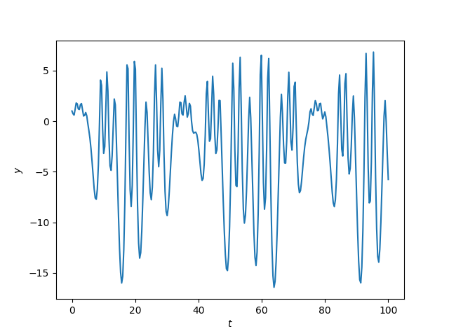
Suppose you have a mass suspended by the combination of a spring and a rubber band. A spring resists being compressed but a rubber band does not. So the rubber band resists motion as the mass moves down but not as it moves up. In [1] the authors use this situation to motivate the following differential equation:

y'' + 0.01 y' + a y^+ - b y^- = 10 + \lambda \sin \mu t

where

\begin{align*} y^+ =& \max\{\phantom{-}y, 0\} \\ y^- =& \max\{-y, 0\} \end{align*}

If ab then we have a linear equation, an ordinary damped, driven harmonic oscillator. But the asymmetry of the behavior of the rubber band causes a and b to be unequal, and that’s what makes the solutions interesting.

For some parameters the system exhibits essentially sinusoidal behavior, but for other parameters the behavior can become chaotic.

Here’s an example of complex behavior.

Motion of mass suspended by spring and rubber band

Here’s the Python code that produced the plot.

    from scipy import linspace, sin
    from scipy.integrate import solve_ivp
    import matplotlib.pyplot as plt

    def pos(x):
        return max(x, 0)

    def neg(x):
        return max(-x, 0)

    a, b, λ, μ = 17, 1, 15.4, 0.75

    def system(t, z):
        y, yp = z # yp = y'
        return [yp, 10 + λ*sin(μ*t) - 0.01*yp - a*pos(y) + b*neg(y)]

    t = linspace(0, 100, 300)

    sol = solve_ivp(system, [0, 100], [1, 0], t_eval=t)
    plt.plot(sol.t, sol.y[0])
    plt.xlabel("$t$")
    plt.ylabel("$y$")

In a recent post I said that I never use non-ASCII characters in programming, so in the code above I did. In particular, it was nice to use λ as a variable; you can’t use lambda as a variable name because it’s a reserved keyword in Python.

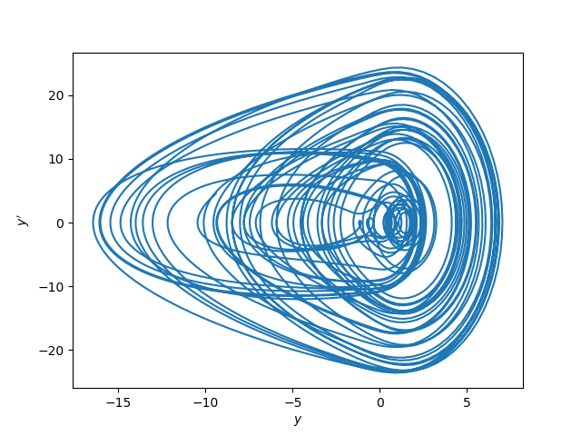
Update: Here’s a phase portrait for the same system.

phase plot

More posts on differential equations

[1] L. D. Humphreys and R. Shammas. Finding Unpredictable Behavior in a Simple Ordinary Differential Equation. The College Mathematics Journal, Vol. 31, No. 5 (Nov., 2000), pp. 338-346

More efficient way to sum a list comprehension

List comprehensions in Python let you create a list declaratively, much like the way you would describe the set in English. For example,

    [x**2 for x in range(10)]

creates a list of the squares of the numbers 0 through 9.

If you wanted the sum of these numbers, you could of course say

    sum( [x**2 for x in range(10)] )

but in this case the brackets are unnecessary. The code is easier to read and more efficient if you omit the brackets.

    sum( x**2 for x in range(10) )

With the brackets, Python constructs the list first then sums the elements. Without the brackets, you have a generator expression. Python will sum the values as they’re generated, not saving all the values in memory. This makes no difference for a short list as above, but with a large list comprehension the generator expression could be more efficient.

Area of sinc and jinc function lobes

Someone left a comment this morning on my blog post on sinc and jinc integrals regarding the area of the lobes.

It would be nice to have the values of integrals of each lobe, i.e. integrals between 0 and multiples of pi. Anyone knows of such a table?

This post will include Python code to address that question. (Update: added asymptotic approximation. See below.)

First, let me back up and explain the context. The sinc function is defined as [1]

sinc(x) = sin(x) / x

and the jinc function is defined analogously as

jinc(x) = J1(x) / x,

substituting the Bessel function J1 for the sine function. You could think of Bessel functions as analogs of sines and cosines. Bessel functions often come up when vibrations are described in polar coordinates, just as sines and cosines come up when using rectangular coordinates.

Here’s a plot of the sinc and jinc functions:

The lobes are the regions between crossings of the x-axis. For the sinc function, the lobe in the middle runs from -π to π, and for n > 0 the nth lobe runs from nπ to (n+1)π. The zeros of Bessel functions are not uniformly spaced like the zeros of the sine function, but they come up in application frequently and so it’s easy to find software to compute their locations.

First of all we’ll need some imports.

    from scipy import sin, pi
    from scipy.special import jn, jn_zeros
    from scipy.integrate import quad

The sinc and jinc functions are continuous at zero, but the computer doesn’t know that [2]. To prevent division by zero, we return the limiting value of each function for very small arguments.

    def sinc(x):
        return 1 if abs(x) < 1e-8 else sin(x)/x

    def jinc(x):
        return 0.5 if abs(x) < 1e-8 else jn(1,x)/x

You can show via Taylor series that these functions are exact to the limits of floating point precision for |x| < 10-8.

Here’s code to compute the area of the sinc lobes.

    def sinc_lobe_area(n):
        n = abs(n)
        integral, info = quad(sinc, n*pi, (n+1)*pi)
        return 2*integral if n == 0 else integral

The corresponding code for the jinc function is a little more complicated because we need to compute the zeros for the Bessel function J1. Our solution is a little clunky because we have an upper bound N on the lobe number. Ideally we’d work out an asymptotic value for the lobe area and compute zeros up to the point where the asymptotic approximation became sufficiently accurate, and switch over to the asymptotic formula for sufficiently large n.

    def jinc_lobe_area(n):
        n = abs(n)
        assert(n < N)
        integral, info = quad(jinc, jzeros[n-1], jzeros[n])
        return 2*integral if n == 0 else integral

Note that the 0th element of the array returned by jn_zeros is the first positive zero of J1; it doesn’t include the zero at the origin.

For both sinc and jinc, the even numbered lobes have positive area and the odd numbered lobes have negative area. Here’s a plot of the absolute values of the lobe areas.

Asymptotic results

We can approximate the area of the nth lobe of the sinc function by using a midpoint approximation for 1/x. It works out that the area is asymptotically equal to

 (-1)^n \frac{4}{(2n+1)\pi}

We can do a similar calculation for the area of the nth jinc lobe, starting with the asymptotic approximation for jinc given here. We find that the area of the nth lobe of the jinc function is asymptotically equal to

\frac{(-1)^n}{\pi^2} \left( \frac{8}{4n+3} \right )^{3/2}

To get an idea of the accuracy of the asymptotic approximations, here are the results for n=100.

    sinc area:      0.00633455
    asymptotic:     0.00633452
    absolute error: 2.97e-8
    relative error: 4.69e-6

    jinc area:      0.000283391
    asymptotic:     0.000283385
    absolute error: 5.66e-9
    relative error: 2.00e-5

More signal processing posts

[1] Some authors define sinc(x) as sin(πx)/πx. Both definitions are common.

[2] Scipy has a sinc function in scipy.special, defined as sin(πx)/πx, but it doesn’t have a jinc function.

Minimizing context switching between shell and Python

Sometimes you’re in the flow using the command line and you’d like to briefly switch over to Python without too much interruption. Or it could be the other way around: you’re in the Python REPL and need to issue a quick shell command.

One solution would be to run your shell and Python session in different terminals, but let’s assume that for whatever reason you’re working in just one terminal. For example, maybe you want the output of a shell command to be visually close when you run Python, or vice versa.

Calling Python from shell

You can run a Python one-liner from the shell by calling Python with the -c option. For example,

    $ python -c "print(3*7)"
    21

I hardly ever do this because I want to run more than a one-liner. What I find more useful is to launch Python with the -q option to suppress all the start-up verbiage and simply bring up a prompt.

    $ python -q
    >>>>

More on this in my post on quiet modes.

Calling shell from Python

If you run Python with the ipython command rather than the default python you get much better shell integration. IPython let’s you type a shell command at any point simply by preceding it with a !. For example, the following command tells us this is the 364th day of the year.

    In [1]: ! date +%j
    364 

You can run some of the most common shell commands, such as cd and ls without even a bang prefix. These are “magic” commands that do what you’d expect if you forgot for a moment that you’re in a Python REPL rather than a command shell.

    In [2]: cd ..
    Out[2]: '/mnt/c/Users'

IPython also supports other forms of shell integration such as capturing the output of a shell command as a Python variable, or using a Python variable as an argument to a shell command.

More on context switching and shells