Engine coolant temperature symbol

My wife and I were talking about the engine coolant temperature symbol on our car dashboard yesterday.

I said I expect there’s a Unicode code point for this symbol. Now I don’t think there is. But there is an ISO Standard name for the symbol. It’s part of ISO 7000: Graphical symbols for use on equipment—Registered symbols, reference number 0246.

A while back I quoted Randall Munroe saying “I am endlessly delighted by the hopeless task that the Unicode Consortium has created for themselves. … These are really hard problems and I do not envy them.” Although the Unicode standard includes an enormous number of symbols, it cannot contain everything.

In my experience the engine coolant temperature symbol is far more common than some of the obscure symbols that have made it into the Unicode standard. One could argue that Unicode should give priority to symbols used in written communication and that symbols like the one above would be low priority. And yet the standard includes many symbols that no one is likely to use in writing. The Unicode Consortium truly does have a hopeless task.

More posts on standards

Privacy implications of hashing data

Cryptographic hash functions are also known as one-way functions because given an input x, one can easily compute its hashed value f(x), but it is impractical to recover x from knowing f(x).

However, if we know that x comes from a small universe of possible values, our one-way function can effectively become a two-way function, i.e. it may be possible to start with f(x) and recover x using a rainbow table attack.

It’s possible to defend against a rainbow attack yet still leak information about the probability distribution of values of x given f(x).

For privacy protection, hashing is better than not hashing. Keyed hashing is better than unkeyed hashing. But even keyed hashing can leak information.

Rainbow tables

Suppose a data set contains SHA-256 hashed values of US Social Security Numbers (SSNs). Since SSNs have 10 digits, there are 10 billion possible SSNs. It would be possible to hash all possible SSNs and create a lookup table, known as a rainbow table. There are three things that make the rainbow table attack possible in this example:

  1. The range of possible inputs is known and relatively small.
  2. The hashing algorithm is known.
  3. The hashing algorithm can be computed quickly.

There are a couple ways to thwart a rainbow table attack. Assuming we have no control of (1) above, we can alter (2) or (3).

Keyed hashing

A way to alter (2) is to use a keyed hash algorithm. For example, if we XOR the SSNs with a key before applying SHA-256, an attacker cannot construct a rainbow table without knowing the key. The attacker may know the core hash algorithm we are using, but they do not know the entire algorithm because the key is part of the algorithm.

Expensive hashing

A way to alter (3) is to use hashing algorithms that are expensive to compute, such as Argon2. The idea is that such hash functions can be computed quickly enough for legitimate use cases, but not for brute-force attacks.

The time required to create a rainbow table is the product of the time to compute a single hash and the size of the set of possible inputs. If it took an hour to compute a hash value, but there are only 10 possible values, then an attacker could compute a rainbow table in 10 hours.

Leaking attribute probabilities

Now suppose we’re using a keyed hashing algorithm. Maybe we’re paranoid and use an expensive hashing algorithm on top of that. What can go wrong now?

If we’re hashing values that each appear one time then we’re OK. If we apply a keyed hash to primary keys in a database, such as patient ID, then the hashed ID does not reveal the patient ID. But if we hash attributes associated with that patient ID, things are different.

Frequency analysis

Suppose US state is an attribute in your database, and you hash this value. No matter how secure and how expensive your hash algorithm is, each state will have a unique hash value. If the database contains a geographically representative sample of the US population, then the hashed state value that appears most often is probably the most populous state, i.e. California. The second most common hashed state value probably corresponds to Texas.

Things are fuzzier on the low end. The hashed state value appearing least often may not correspond to Wyoming, but it very likely does not correspond to Florida, for example.

In short, you can infer the state values using the same kind of frequency analysis you’d use to solve a simple substitution cipher in a cryptogram puzzle. The larger the data set, the more closely the empirical order will likely align with the population order.

Maybe this is OK?

Frequency analysis makes it possible to infer (with some uncertainty) the most common values. But the most common values are also the least informative. Knowing someone is from California narrows down their identity less than knowing that they are from Wyoming.

Frequency analysis is less specific for less common values. It might not tell you with much confidence that someone is from Wyoming, but it might tell you with some confidence that they come from a low-population state. However, since there are several low-population states, knowing someone is from such a state, without knowing which particular state, isn’t so informative.

Data privacy depends on context. Knowing what state someone is likely from may or may not be a problem depending on what other information is available.

Related posts

Topological sort

When I left academia [1] my first job was working as a programmer. I was very impressed by a new programmer we hired who hit the ground running. His first week he looked at some problem we were working on and said “Oh, you need a topological sort.” I’d never heard of a topological sort and it sounded exotic. What could this have to do with topology?!

A topological sort of a directed graph lists source nodes before target nodes. For example, if there is a directed edge from A to B and from C to A, then the nodes would be list C, A, B. It’s just a way of listing items in a directed graph so that no item in the list points to an item earlier in the list. All arrows point forward.

This is not exotic at all. It’s something you’ve likely done, maybe by hand. As pointed out in the comments, the make utility does this, compiling source files in the order that they’re needed [2].

Where does topology come in? Imagine your directed graph made of beads and strings. You want to pick up the graph by some bead so that all beads are higher than the beads they point to. It’s topological in the sense that you don’t need to preserve the geometry of the graph, only its connectivity.

tsort

The Unix utility tsort will do a topological sort. The input to the utility is a text file with two items per line, separated by white space, indicating a directed edge from the first item to the second.

Example

Here is a thumbnail image of a graph of relationships between special functions. See this page for a full-sized image and an explanation of what the arrows represent.

special function relationships

I took the GraphViz file used to create the graph and formatted it for tsort. Then I randomly shuffled the file with shuf.

    Gegenbauer_polynomials Legendre_polynomials
    Gegenbauer_polynomials Chebyshev_polynomials_Second_kind
    Hypergeometric_2F1 Jacobi_polynomials
    Error_function Fresnel_S
    ...
    Hypergeometric_1F1 Error_function

The lines are not sorted topologically because, for example, the Gegenbauer polynomials are special cases of the Hypergeometric 2F1 functions, so Hypergeometric 2F1 should be listed before Gegenbauer polynomials.

When I ran the shuffled file through tsort I got

    Elliptic_F
    Hypergeometric_2F1
    Elliptic_E
    Hypergeometric_1F1
    ....
    Beta

and now in this list more general functions always come before special cases.

Related posts

[1] After a postdoc at Vanderbilt, I took a job as a programmer. I got the job because they needed a programmer who knew some DSP. A few years later I got a job at MD Anderson Cancer Center managing a group of programmers. It’s fuzzy whether my time at MDACC should be considered time in Academia. My responsibilities there were sometimes academic—writing journal articles, teaching classes—and sometimes not—developing software and managing software developers.

[2] The make software can be used to run any directed acyclic graph of tasks, but is most often used to compile software.

“We won’t sell your personal data, but …”

When a company promises not to sell your personal data, this promise alone doesn’t mean much.

“We will not sell your personal data, but …

  • We might get hacked.
  • We might give it to a law enforcement or intelligence agency.
  • We might share or trade your data without technically selling it.
  • We might alter our terms. Pray we do not alter them any further.
  • We might be acquired by a new company that alters the terms.
  • We might go bankrupt and the data be sold as an asset.”


(This post started as a Twitter thread. Thanks to Michael Madden for his contribution to the thread.)

Connecting the dots differently

A couple weeks ago I wrote about how H. A. Rey introduced a new way of looking at the constellations, making them look more like their names. That post used Leo as an example. This post looks at Boötes (The Herdsman) [1].

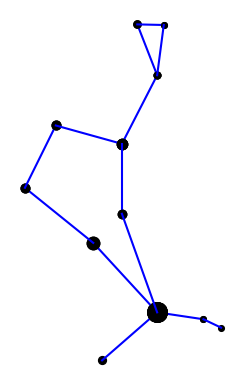
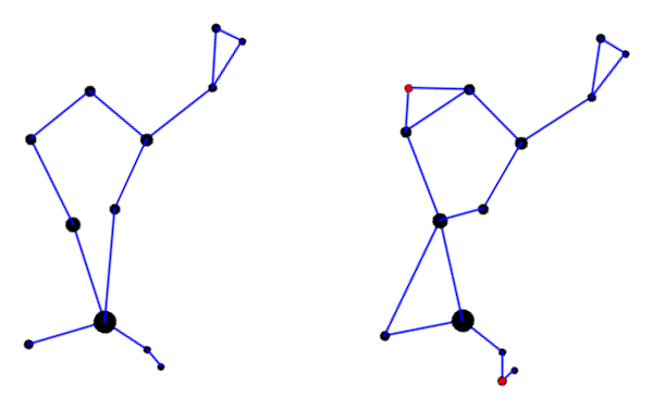
Here is the constellation using the connections indicated in the IAU star chart.

Bootes from IAU chart

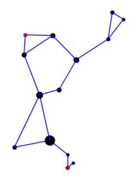
Here is the constellation using the connections drawn in Rey’s book [2].

H. A. Rey's version of Bootes

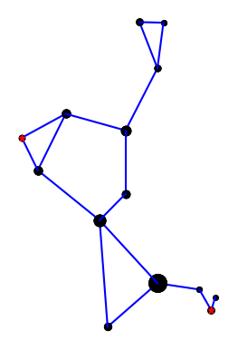
Rey’s version adds two stars, highlighted in red, but mostly connects the same stars in a different way. I suppose the herdsman is standing in the IAU version; it’s hard to tell. In Rey’s version, the huntsman is clearly seated and smoking a pipe. This is easier to see if we rotate the image a bit.

Rey's herdsman, rotated

Here’s a comparison of the two interpretations side-by-side.

comparing both versions

Here is the Python code that produced the two images. It’s a little cleaner than the code in the earlier post, and it draws larger dots to represent brighter stars.

import matplotlib.pyplot as plt

# data from https://en.wikipedia.org/wiki/List_of_stars_in_Bo%C3%B6tes

α = (14 + 16/60, 19 + 11/60, 0.0)  
β = (15 +  2/60, 40 + 23/60, 3.5)  
γ = (14 + 32/60, 38 + 18/60, 3.0)  
δ = (15 + 16/60, 33 + 19/60, 3.5)  
ε = (14 + 45/60, 27 +  4/60, 2.3)  
ζ = (14 + 41/60, 13 + 44/60, 3.8)  
η = (13 + 55/60, 18 + 24/60, 4.5)  
θ = (14 + 25/60, 51 + 51/60, 4.0)  
κ = (14 + 13/60, 51 + 47/60, 4.5)  
λ = (14 + 16/60, 46 +  5/60, 4.2)
μ = (15 + 24/60, 37 + 23/60, 4.3)
υ = (13 + 49/60, 15 + 48/60, 4.0)  
τ = (13 + 47/60, 17 + 27/60, 4.5)  
ρ = (14 + 32/60, 30 + 22/60, 3.6)  
    
k = -15 # reverse and scale horizontal axis

def plot_star(s, m):
    plt.plot(k*s[0], s[1], m, markersize=14-2.2*s[2])    

def join(s0, s1, m='ko'):
    plot_star(s0, m)
    plot_star(s1, m)    
        
    plt.plot([k*s0[0], k*s1[0]], [s0[1], s1[1]], 'b-')    

def draw_iau():

    join(α, η)
    join(η, τ)
    join(α, ζ)
    join(α, ϵ)
    join(ϵ, δ)
    join(δ, β)
    join(β, γ)
    join(γ, λ)
    join(λ, θ)
    join(θ, κ)
    join(κ, λ)
    join(γ, ρ)
    join(ρ, α)

def draw_rey():

    join(α, η)
    join(η, υ)
    join(υ, τ)
    
    join(α, ζ)
    join(α, ϵ)
    join(ζ, ϵ)
    
    join(ϵ, δ)
    join(δ, β)
    join(δ, μ)
    join(μ, β)
    join(β, γ)
    join(γ, λ)
    join(λ, θ)
    join(θ, κ)
    join(κ, λ)
    join(γ, ρ)
    join(ρ, ϵ)

    plot_star(μ, 'r*')
    plot_star(υ, 'r*')        
    return

draw_iau()
plt.gca().set_aspect('equal')
plt.axis('off')
plt.savefig("bootes_iau.png")
plt.close()

draw_rey()
plt.gca().set_aspect('equal')
plt.axis('off')
plt.savefig("bootes_rey.png")
plt.close()

***

[1] The diaeresis over the second ‘o’ in Boötes means the two vowels are to be pronounced separately: bo-OH-tes. You may have seen the same pattern in Laocoön or oogenesis. The latter is written without a diaeresis now, but I bet authors used to write it with a diaeresis on the second ‘o’.

[2] H. A. Rey. The Stars: A New Way to See Them, Second Edition.

Famous constants and the Gumbel distribution

The Gumbel distribution, named after Emil Julius Gumbel (1891–1966), is important in statistics, particularly in studying the maximum of random variables. It comes up in machine learning in the so-called Gumbel-max trick. It also comes up in other applications such as in number theory.

For this post, I wanted to point out how a couple famous constants are related to the Gumbel distribution.

Gumbel distribution

The standard Gumbel distribution is most easily described by its cumulative distribution function

F(x) = exp( −exp(−x) ).

You can introduce a location parameter μ and scale parameter β the usual way, replacing x with (x − μ)/β and dividing by β.

Here’s a plot of the density.

Euler-Mascheroni constant γ

The Euler-Mascheroni constant γ comes up frequently in applications. Here are five posts where γ has come up.

The constant γ comes up in the context of the Gumbel distribution two ways. First, the mean of the standard Gumbel distribution is γ. Second, the entropy of a standard Gumbel distribution is γ + 1.

Apéry’s constant ζ(3)

The values of the Riemann zeta function ζ(z) at positive even integers have closed-form expressions given here, but the values at odd integers do not. The value of ζ(3) is known as Apéry’s constant because Roger Apéry proved in 1978 that ζ(3) is irrational.

Like the Euler-Mascheroni constant, Apéry’s constant has come up here multiple times. Some examples:

The connection of the Gumbel distribution to Apéry’s constant is that the skewness of the distribution is

12√6 ζ(3)/π³.

Strengthen Markov’s inequality with conditional probability

Markov’s inequality is very general and hence very weak. Assume that X is a non-negative random variable, a > 0, and X has a finite expected value, Then Markov’s inequality says that

\text{P}(X > a) \leq \frac{\text{E}(X)}{a}

In [1] the author gives two refinements of Markov’s inequality which he calls Hansel and Gretel.

Hansel says

\text{P}(X > a) \leq \frac{\text{E}(X)}{a + \text{E}(X - a \mid X > a)}

and Gretel says

\text{P}(X > a) \leq \frac{\text{E}(X) - \text{E}(X \mid X \leq a)}{a - \text{E}(X \mid X \leq a)}

Related posts

[1] Joel E. Cohen. Markov’s Inequality and Chebyshev’s Inequality for Tail Probabilities: A Sharper Image. The American Statistician, Vol. 69, No. 1 (Feb 2015), pp. 5-7

There’s a woset in my reposit

The other day I was talking with someone I met while I was doing my postdoc at Vanderbilt and Eric Schechter’s book Handbook of Analysis and its Foundations came up. Eric was writing that book while we were there. He kindly listed me in the acknowledgements for having reviewed a few pages of the book.

I was curious how the book turned out and so I borrowed a copy through my local library. I was thumbing through the book and saw that Eric used woset as an abbreviation for well-ordered set. If I had seen that before, it made no impression on me. But since that time I have read There’s a Wocket in My Pocket aloud to four children, and so now my Pavlovian response to hearing “woset” is to think “in my closet.”

The context of the line is

“Did you ever have a feeling there’s a WASKET in your BASKET?

… Or a NUREAU in your BUREAU?

… Or a WOSET in your CLOSET?”

If I remember correctly, Eric started out to write a book about partial differential equations and worked his way backward to foundational theorems from analysis and logic. The end of the book discusses analytic semigroups, important in the theory of parabolic PDEs, but the large majority of the book is a repository of abstract analysis.

Solid angle of a star

The apparent size of a distant object can be measured by projecting the object onto a unit sphere around the observer and calculating the area of the projected image.

A unit sphere has area 4π. If you’re in a ship far from land, the solid angle of the sky is 2π steradians because it takes up half a sphere.

If the object you’re looking at is a sphere of radius r whose center is a distance d away, then its apparent size is

\Omega = 2\pi\left(1 - \frac{\sqrt{d^2 - r^2}}{d}\right)

steradians. This formula assumes d > r. Otherwise you’re not looking out at the sphere; you’re inside the sphere.

If you’re looking at a star, then d is much larger than r, and we can simplify the equation above. The math is very similar to the math in an earlier post on measuring tapes. If you want to measure the size of a room, and something is blocking you from measuring straight from wall to wall, it doesn’t make much difference if the object is small relative to the room. It all has to do with Taylor series and the Pythagorean theorem.

Think of the expression above as a function of r and expand it in a Taylor series around r = 0.

\Omega = 2\pi\left(1 - \frac{\sqrt{d^2 - r^2}}{d}\right) = 2\pi\left(\frac{\sqrt{r^2}}{2d^2} + \frac{r^4}{8d^4} + \cdots \right)

and so

\Omega \approx \frac{\pi r^2}{d^2}

with an error on the order of (r/d)4. To put it another way, the error in our approximation for Ω is on the order of Ω². The largest object in the sky is the sun, and it has apparent size less than 10−4, so Ω is always small when looking at astronomical objects, and Ω² is negligible.

So for practical purposes, the apparent size of a celestial object is π times the square of the ratio of its radius to its distance. This works fine for star gazing. The approximation wouldn’t be as accurate for watching a hot air balloon launch up close.

Square degrees

Sometimes solid angles are measured in square degrees, given by π/4 times the square of the apparent diameter in degrees. This implicitly uses the approximation above since the apparent radius is r/d.

(The area of a square is diameter squared, and a circle takes up π/4 of a square.)

Examples

When I typed

    3.1416 (radius of sun / distance to sun)^2

into Wolfram Alpha I got 6.85 × 10⁻⁵. (When I used “pi” rather than 3.1416 it interpreted this as the radius of a pion particle.)

When I typed

    3.1416 (radius of moon / distance to moon)^2

I got 7.184 × 10⁻⁵, confirming that the sun and moon are approximately the same apparent size, which makes a solar eclipse possible.

The brightest star in the night sky is Sirius. Asking Wolfram Alpha

    3.1416 (radius of Sirius / distance to Sirius)^2

we get 6.73 × 10⁻¹⁶.

Related posts

Fixed points of the Fourier transform

This previous post looked at the hyperbolic secant distribution. This distribution has density

f_H(x) = \frac{1}{2} \text{sech} \left(\frac{\pi x}{2} \right)

and characteristic function sech(t). It’s curious that the density and characteristic function are so similar.

The characteristic function is essentially the Fourier transform of the density function, so this says that the hyperbolic secant function, properly scaled, is a fixed point of the Fourier transform. I’ve long known that the normal density is its own Fourier transform, but only recently learned that the same is true of the hyperbolic secant.

Hermite functions

The Hermite functions are also fixed points of the Fourier transform, or rather eigenfunctions of the Fourier transform. The eigenvalues are 1, i, -1, and i. When the eigenvalues are 1, we have fixed points.

There are two conventions for defining the Hermite functions, and multiple conventions for defining the Fourier transform, so the truth of the preceding paragraph depends on the conventions used.

For this post, we will define the Fourier transform of a function f to be

\hat{f}(\omega) = \frac{1}{\sqrt{2\pi}} \int_{-\infty}^\infty \exp(-i \omega x)\, f(x)\, dx

Then the Fourier transform of exp(-x²/2) is the same function. Since the Fourier transform is linear, this means the same holds for the density of the standard normal distribution.

We will define the Hermite polynomials by

H_n(x) = (-1)^n e^{x^2}\frac{d^n}{dx^n}e^{-x^2}

using the so-called physics convention. Hn is an nth degree polynomial.

The Hermite functions ψn(x) are the Hermite polynomials multiplied by exp(-x²/2). That is,

\psi_n(x) = H_n(x) \exp(-x^2/2)

With these definitions, the Fourier transform of ψn(x) equals (-i)n ψn(x). So when n is a multiple of 4, the Fourier transform of ψn(x) is ψn(x).

[The definition Hermite functions above omits a complicated constant term that depends on n but not on x. So our Hermite functions are proportional to the standard Hermite functions. But proportionality constants don’t matter when you’re looking for eigenfunctions or fixed points.]

Hyperbolic secant

Using the definition of Fourier transform above, the function sech(√(π/2) x) is its own Fourier transform.

This is surprising because the Hermite functions form a basis for L²(ℝ), and all have tails on the order of exp(-x²), but the hyperbolic secant has tails like exp(-x). Each Hermite function eventually decays like exp(-x²), but this happens later as n increases, so an infinite sum of Hermite functions can have thicker tails than any particular Hermite function.

Related posts