Number of forms of a finite field

The number of elements in a finite field must be a prime power, and for every prime power there is only one finite field up to isomorphism.

The finite field with 256 elements, GF(28), is important in applications. From one perspective, there is only one such field. But there are a lot of different isomorphic representations of that field, and some are more efficient to work with that others.

Just how many ways are there to represent GF(28)? Someone with the handle joriki gave a clear answer on Stack Exchange:

There are 28−1 different non-zero vectors that you can map the first basis vector to. Then there are 28−2 different vectors that are linearly independent of that vector that you can map the second basis vector to, and so on. In step k, 2k-1 vectors are linear combinations of the basis vectors you already have, so 28−2k−1 aren’t, so the total number of different automorphisms is

\prod_{k=1}^8\left(2^8 - 2^{k-1} \right ) = 5348063769211699200

This argument can be extended to count the number of automorphism of any finite field.

More finite field posts

Area of sinc and jinc function lobes

Someone left a comment this morning on my blog post on sinc and jinc integrals regarding the area of the lobes.

It would be nice to have the values of integrals of each lobe, i.e. integrals between 0 and multiples of pi. Anyone knows of such a table?

This post will include Python code to address that question. (Update: added asymptotic approximation. See below.)

First, let me back up and explain the context. The sinc function is defined as [1]

sinc(x) = sin(x) / x

and the jinc function is defined analogously as

jinc(x) = J1(x) / x,

substituting the Bessel function J1 for the sine function. You could think of Bessel functions as analogs of sines and cosines. Bessel functions often come up when vibrations are described in polar coordinates, just as sines and cosines come up when using rectangular coordinates.

Here’s a plot of the sinc and jinc functions:

The lobes are the regions between crossings of the x-axis. For the sinc function, the lobe in the middle runs from -π to π, and for n > 0 the nth lobe runs from nπ to (n+1)π. The zeros of Bessel functions are not uniformly spaced like the zeros of the sine function, but they come up in application frequently and so it’s easy to find software to compute their locations.

First of all we’ll need some imports.

    from scipy import sin, pi
    from scipy.special import jn, jn_zeros
    from scipy.integrate import quad

The sinc and jinc functions are continuous at zero, but the computer doesn’t know that [2]. To prevent division by zero, we return the limiting value of each function for very small arguments.

    def sinc(x):
        return 1 if abs(x) < 1e-8 else sin(x)/x

    def jinc(x):
        return 0.5 if abs(x) < 1e-8 else jn(1,x)/x

You can show via Taylor series that these functions are exact to the limits of floating point precision for |x| < 10-8.

Here’s code to compute the area of the sinc lobes.

    def sinc_lobe_area(n):
        n = abs(n)
        integral, info = quad(sinc, n*pi, (n+1)*pi)
        return 2*integral if n == 0 else integral

The corresponding code for the jinc function is a little more complicated because we need to compute the zeros for the Bessel function J1. Our solution is a little clunky because we have an upper bound N on the lobe number. Ideally we’d work out an asymptotic value for the lobe area and compute zeros up to the point where the asymptotic approximation became sufficiently accurate, and switch over to the asymptotic formula for sufficiently large n.

    def jinc_lobe_area(n):
        n = abs(n)
        assert(n < N)
        integral, info = quad(jinc, jzeros[n-1], jzeros[n])
        return 2*integral if n == 0 else integral

Note that the 0th element of the array returned by jn_zeros is the first positive zero of J1; it doesn’t include the zero at the origin.

For both sinc and jinc, the even numbered lobes have positive area and the odd numbered lobes have negative area. Here’s a plot of the absolute values of the lobe areas.

Asymptotic results

We can approximate the area of the nth lobe of the sinc function by using a midpoint approximation for 1/x. It works out that the area is asymptotically equal to

 (-1)^n \frac{4}{(2n+1)\pi}

We can do a similar calculation for the area of the nth jinc lobe, starting with the asymptotic approximation for jinc given here. We find that the area of the nth lobe of the jinc function is asymptotically equal to

\frac{(-1)^n}{\pi^2} \left( \frac{8}{4n+3} \right )^{3/2}

To get an idea of the accuracy of the asymptotic approximations, here are the results for n=100.

    sinc area:      0.00633455
    asymptotic:     0.00633452
    absolute error: 2.97e-8
    relative error: 4.69e-6

    jinc area:      0.000283391
    asymptotic:     0.000283385
    absolute error: 5.66e-9
    relative error: 2.00e-5

More signal processing posts

[1] Some authors define sinc(x) as sin(πx)/πx. Both definitions are common.

[2] Scipy has a sinc function in scipy.special, defined as sin(πx)/πx, but it doesn’t have a jinc function.

Doing a database join with CSV files

relational database

It’s easy to manipulate CSV files with basic command line tools until you need to do a join. When your data is spread over two different files, like two tables in a normalized database, joining the files is more difficult unless the two files have the same keys in the same order. Fortunately, the xsv utility is just the tool for the job. Among other useful features, xsv supports database-like joins.

Suppose you want to look at weights broken down by sex, but weights are in one file and sex is in another. The weight file alone doesn’t tell you whether the weights belong to men or women.

Suppose a file weight.csv has the following rows:

    ID,weight
    123,200
    789,155
    999,160

and a file person.csv has the following:

    ID,sex
    123,M
    456,F
    789,F

Note that the two files have different ID values: 123 and 789 are in both files, 999 is only in weight.csv and 456 is only in person.csv. We want to join the two tables together, analogous to the JOIN command in SQL.

The command

    xsv join ID person.csv ID weight.csv

does just this, producing

    ID,sex,ID,weight
    123,M,123,200
    789,F,789,155

by joining the two tables on their ID columns.

The command includes ID twice, once for the field called ID in person.csv and once for the field called ID in weight.csv. The fields could have different names. For example, if the first column of person.csv were renamed Key, then the command

    xsv join Key person.csv ID weight.csv

would produce

    Key,sex,ID,weight
    123,M,123,200
    789,F,789,155

We’re not interested in the ID columns per se; we only want to use them to join the two files. We could suppress them in the output by asking xsv to select the second and fourth columns of the output

    xsv join Key person.csv ID weight.csv | xsv select 2,4

which would return

    sex,weight
    M,200
    F,155

We can do other kinds of joins by passing a modifier to join. For example, if we do a left join, we will include all rows in the left file, person.csv, even if there isn’t a match in the right file, weight.csv. The weight will be missing for such records, and so

    $ xsv join --left Key person.csv ID weight.csv

produces

    Key,sex,ID,weight
    123,M,123,200
    456,F,,
    789,F,789,155

Right joins are analogous, including every record from the second file, and so

    xsv join --right Key person.csv ID weight.csv

produces

    Key,sex,ID,weight
    123,M,123,200
    789,F,789,155
    ,,999,160

You can also do a full join, with

    xsv join --full Key person.csv ID weight.csv

producing

    Key,sex,ID,weight
    123,M,123,200
    456,F,,
    789,F,789,155
    ,,999,160

More data wrangling posts

Exporting Excel files to CSV with in2csv

This post shows how to export an Excel file to a CSV file using in2csv from the csvkit package.

You could always use Excel itself to export an Excel file to CSV but there are several reasons you might not want to. First and foremost, you might not have Excel. Another reason is that you might want to work from the command line in order to automate the process. Finally, you might not want the kind of CSV format that Excel exports.

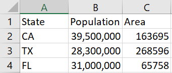
For illustration I made a tiny Excel file. In order to show how commas are handled, populations contain commas but areas do not.

See post content for text dump of data

When I ask Excel to export the file I get

    State,Population,Area
    CA,"39,500,000",163695
    TX,"28,300,000",268596
    FL,"31,000,000",65758

Note that areas are exported as plain integers, but populations are exported as quoted strings containing commas.

Using csvkit

Now install csvkit and run in2csv.

    $ in2csv states.xlsx
    State,Population,Area
    CA,39500000,163695
    TX,28300000,268596
    FL,31000000,65758

The output goes to standard out, though of course you could redirect the output to a file. All numbers are exported as numbers, with no thousands separators. This makes the output easier to use from a program that does crude parsing [1]. For example, suppose we save states.xlsx to states.csv using Excel then ask cut for the second column. Then we don’t get what we want.

    $ cut -d, -f2 states.csv
    Population
    "39
    "28
    "31

But if we use in2csv to create states.csv then we get what we’d expect.

    cut -d, -f2 states.csv
    Population
    39500000
    28300000
    31000000

Multiple sheets

So far we’ve assumed our Excel file has a single sheet. I added a second sheet with data on US territories. The sheet doesn’t have a header row just to show that the header row isn’t required.

PR\t3,300,000\t5325\nGuam\t161,700\t571

I named the two sheets “States” and “Territories” respectively.

States, Territories

Now if we ask in2csv to export our Excel file as before, it only exports the first sheet. But if we specify the Territories sheet, it will export that.

    $ in2csv --sheet Territories states.xlsx
    PR,3300000,5325
    Guam,161700,571

More CSV posts

[1] The cut utility isn’t specialized for CSV files and doesn’t understand that commas inside quotation marks are not field separators. A specialized utility like csvtool would make this distinction. You could extract the second column with

    csvtool col 2 states.csv

or

    csvtool namedcol Population states.csv

This parses the columns correctly, but you still have to remove the quotation marks and thousands separators.

Minimizing context switching between shell and Python

Sometimes you’re in the flow using the command line and you’d like to briefly switch over to Python without too much interruption. Or it could be the other way around: you’re in the Python REPL and need to issue a quick shell command.

One solution would be to run your shell and Python session in different terminals, but let’s assume that for whatever reason you’re working in just one terminal. For example, maybe you want the output of a shell command to be visually close when you run Python, or vice versa.

Calling Python from shell

You can run a Python one-liner from the shell by calling Python with the -c option. For example,

    $ python -c "print(3*7)"
    21

I hardly ever do this because I want to run more than a one-liner. What I find more useful is to launch Python with the -q option to suppress all the start-up verbiage and simply bring up a prompt.

    $ python -q
    >>>>

More on this in my post on quiet modes.

Calling shell from Python

If you run Python with the ipython command rather than the default python you get much better shell integration. IPython let’s you type a shell command at any point simply by preceding it with a !. For example, the following command tells us this is the 364th day of the year.

    In [1]: ! date +%j
    364 

You can run some of the most common shell commands, such as cd and ls without even a bang prefix. These are “magic” commands that do what you’d expect if you forgot for a moment that you’re in a Python REPL rather than a command shell.

    In [2]: cd ..
    Out[2]: '/mnt/c/Users'

IPython also supports other forms of shell integration such as capturing the output of a shell command as a Python variable, or using a Python variable as an argument to a shell command.

More on context switching and shells

A new take on the birthday problem

Vitalii Tymchyshyn and Andrii Khlevniuk posted a new paper here entitled “On the average number of birthdays in birthday paradox setup.” This paper gives a different perspective on the birthday problem and a new proof.

In the usual formation of the birthday problem, one asks the probability that everyone in a group of size n has a different birthday, or one asks how big n needs to be for the probability to be approximately 1/2 that two people share a birthday. Tymchyshyn and Khlevniuk ask about the expected number of unique birthdays in a group of size n and show that it equals

(1 – αn) / (1 – α)

where α = 364/365.

Variations on the birthday problem often come up in practice. For example, you often need to consider how likely it is that a hash function will map set of inputs to unique values. There’s a rule of thumb that if there are N possible hash values, then there’s a 50-50 chance of a collision if you hash √N values.

Let α = (N-1)/N and p = 1/N. If we take the first three terms in the Taylor series for (1 – p)n we see that the expected number of unique hash values after hashing n inputs is approximately

nn(n – 1) p/2.

If we choose n = √N, then the expected number of unique hash values is approximately

n – 1/2,

which is consistent with having about a 0.5 probability of one collision.

Related probability posts

Driven Van der Pol oscillators

I’ve playing around with driven Van der Pol oscillators.

{d^2x \over dt^2}= \mu(1-x^2){dx \over dt}- x + F \cos(2\pi t/T)

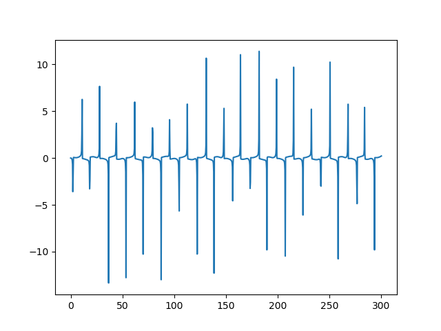
The cosine term is the driving function. You can see a variety of behavior depending on the interaction between the driving frequency and the natural frequency, along with the other parameters. Sometimes you get periodic solutions and sometimes you get chaotic behavior.

Here’s the Python code I started with

    a, b = 0, 300
    t = linspace(a, b, 1000)
    mu = 9
    T = 10

    def vdp_driven(t, z):
        x, y = z
        return [y, mu*(1 - x**2)*y - x + cos(2*pi*t/T)]
    
    sol = solve_ivp(vdp_driven, [a, b], [1, 0], t_eval=t)
    plt.plot(sol.y[0], sol.y[1])

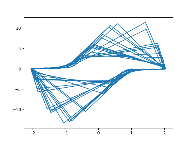
The first phase plot looked like this:

low res phase plot

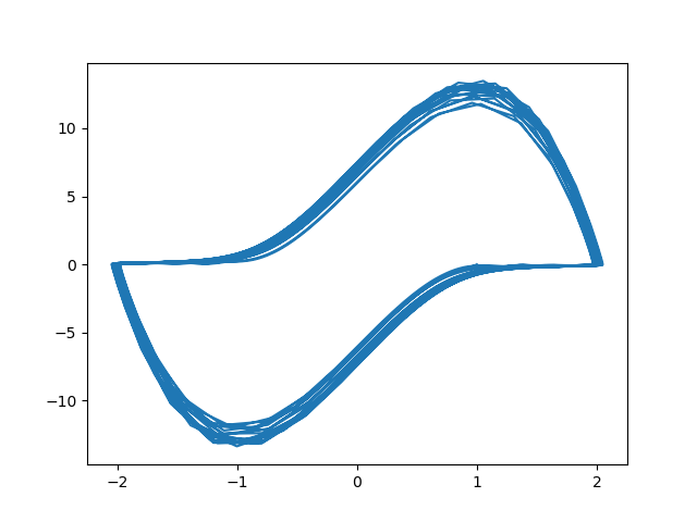
That’s weird. So I increased the number of solution points by changing the last argument to linspace from 1,000 to 10,000. Here’s the revised plot.

low res phase plot

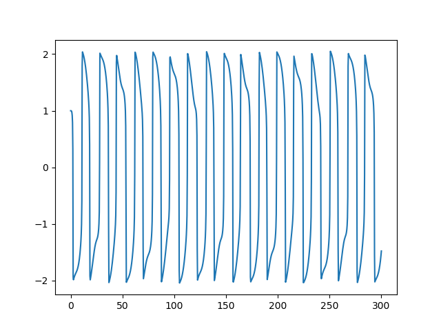
That’s a lot different. What’s going on? The solutions to the driven Van der Pol equation, and especially their derivative, change abruptly, so abruptly that if there’s not an integration point in the transition zone you get the long straight lines you see above. With more resolution these lines go away. This is understandable when you look at the plot of the solution:

low res phase plot

and of its derivative:

low res phase plot

The solution looks fairly regular but the varying amplitudes of the derivative highlight the irregular behavior. The correct phase plot is not as crazy as the low-resolution version suggests, but we can see that the solution does not quickly settle into a limit cycle as it does in the undriven case.

More Van der Pol posts

Calculating the period of Van der Pol oscillators

A few days ago I wrote about how to solve differential equations with SciPy’s ivp_solve function using Van der Pol’s equation as the example. Van der Pol’s equation is

{d^2x \over dt^2}-\mu(1-x^2){dx \over dt}+x= 0

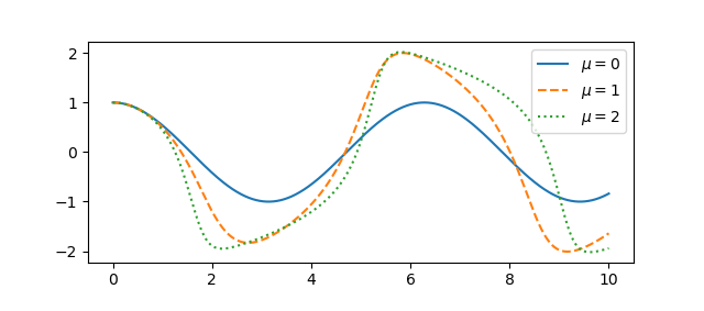
The parameter μ controls the amount of nonlinear damping. For any initial condition, the solution approach a periodic solution. The limiting periodic function does not depend on the initial condition [1] but does depend on μ. Here are the plots for μ  = 0, 1, and 2 from the previous post.

Van der Pol oscillator solutions as a function of time

A couple questions come to mind. First, how quickly do the solutions become periodic? Second, how does the period depend on μ? To address these questions, we’ll use an optional argument to ivp_solve we didn’t need in the earlier post.

Using events in ivp_solve

For ivp_solve an event is a function of the time t and the solution y whose roots the solver will report. To determine the period, we’ll look at where the solution is zero; our event function is trivial since we want to find the roots of the solution itself.

Recall from the earlier post that we cast our second order ODE as a pair of first order ODEs, and so our solution is a vector, the function x and its derivative. So to find roots of the solution, we look at what the solver sees as the first component of the solver. So here’s our event function:

    def root(t, y): return y[0]

Let’s set μ = 2 and find the zeros of the solution over the interval [0, 40], starting from the initial condition x(0) = 1, x‘(0) = 0.

    mu = 2
    sol = solve_ivp(vdp, [0, 40], [1, 0], events=root)
    zeros = sol.t_events[0]

Here we reuse the vdp function from the previous post about the Van der Pol oscillator.

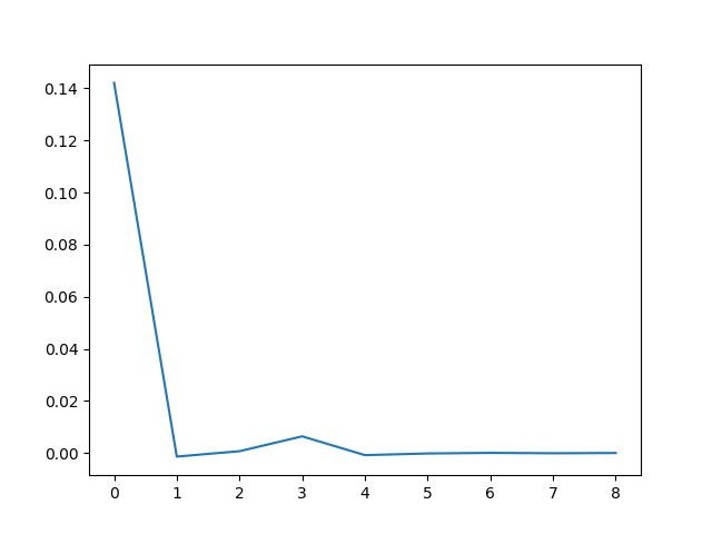
To estimate the period of the limit cycle we look at the spacing between zeros, and how that spacing is changing.

    spacing = zeros[1:] - zeros[:-1]
    deltas = spacing[1:] - spacing[:-1]

If we plot the deltas we see that the zero spacings quickly approach a constant value. Zero crossings are half periods, so the period of the limit cycle is twice the limiting spacing between zeros.

Van der pol period deltas

Theoretical results

If μ = 0 the Van der Pol oscillator reduces to a simple harmonic oscillator and the period is 2π. As μ increases, the period increases.

For relatively small μ we can calculate the period as above, but as μ increases this becomes more difficult numerically [2]. But one can easily show that the period is asymptotically

T ~ (3 – 2 log 2) μ

as μ goes to infinity. A more refined estimate due to Mary Cartwright is

T ~ (3 – 2 log 2) μ + 2π/μ1/3

for large μ.

More VdP posts

[1] There is a trivial solution, x = 0, corresponding to the initial conditions x(0) = x‘(0) = 0. Otherwise, every set of initial conditions leads to a solution that converges to the periodic attractor.

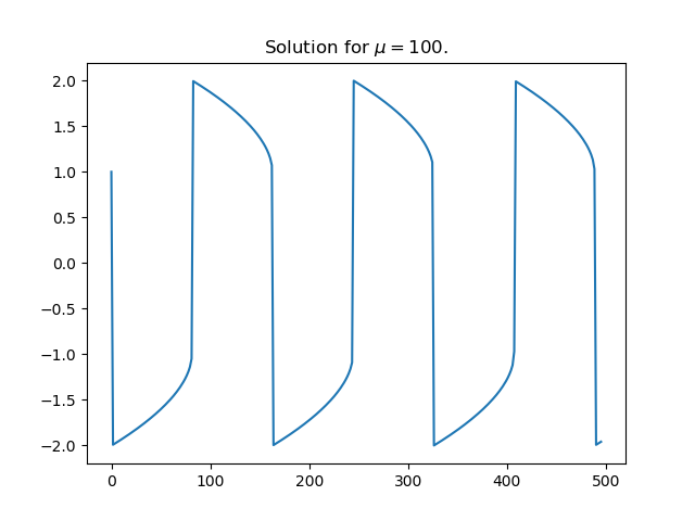
[2] To see why large values of μ are a problem numerically, here’s a plot of a solution for μ = 100.

Solution to Van der Pol for large damping parameter mu

The solution is differentiable everywhere, but the derivative changes so abruptly at the maxima and minima that it is discontinuous for practical purposes.

Master / Apprentice relationship graph in Star Wars

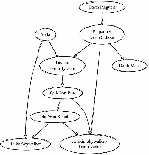
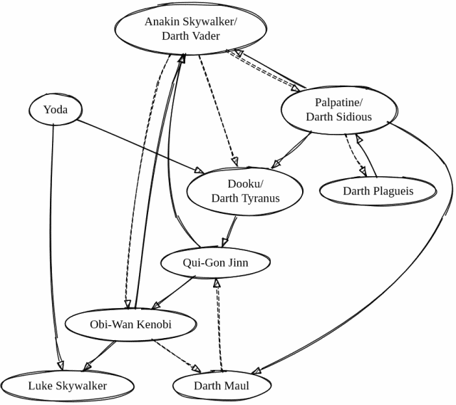
Here’s a graph of master / apprentice relationships for Jedi and Sith in the Star Wars movies. It’s not exhaustive, but it covers the main relationships in Episodes I through VI.

Jedi master/padawan relationships

Here’s what you get if you add a dashed arrow for who killed whom.

Master / apprentice relationships with who killed whom

Here’s the dot (GraphVis) code that created the diagrams.

digraph G {

    Vader [label="Anakin Skywalker/\nDarth Vader"];
    Dooku [label="Dooku/\nDarth Tyranus"];
    Luke  [label="Luke Skywalker"];
    Ben   [label="Obi-Wan Kenobi"];
    Liam  [label="Qui-Gon Jinn"];
    DS    [label="Palpatine/\nDarth Sidious"]
    DP    [label="Darth Plagueis"];
    DM    [label="Darth Maul"];

    Yoda  -> Dooku;
    Yoda  -> Luke;
    Dooku -> Liam;
    Liam  -> Ben;
    Liam  -> Vader;
    Ben   -> Vader;
    Ben   -> Luke;
    DS    -> Dooku;
    DS    -> Vader;
    DP    -> DS;
    DS    -> DM;
    
    Vader -> DS [style=dashed];
    Vader -> Dooku [style=dashed];
    Vader -> Ben [style=dashed];
    Ben   -> DM [style=dashed];    
    DM    -> Liam [style=dashed];
    DS    -> DP [style=dashed];
}

More network visualization posts