Entropy of a Student t distribution

I was looking up the entropy of a Student t distribution and something didn’t seem right, so I wanted to look at familiar special cases.

The Student t distribution with ν degrees of freedom has two important special cases: ν = 1 and ν = ∞. When ν = 1 we get the Cauchy distribution, and in the limit as ν → ∞ we get the normal distribution. The expression for entropy is simple in these two special cases, but it’s not at all obvious that the general expression at ν = 1 and ν = ∞ gives the entropy for the Cauchy and normal distributions.

The entropy of a Cauchy random variable (with scale 1) is

\log(4 \pi)

and the entropy of a normal random variable (with scale 1) is

(\log(2\pi) + 1)/2

The entropy of a Student t random variable with ν degrees of freedom is

\frac{\nu+1}{2} \left( \psi\left(\frac{\nu + 1}{2}\right) - \psi\left(\frac{\nu}{2}\right) \right) + \log\left( \sqrt{\nu} B\left(\frac{\nu}{2}, \frac{1}{2} \right) \right)

Here ψ is the digamma function, the derivative of the log of the gamma function, and B is the beta function. These two functions are implemented as psi and beta in Python, and PolyGamma and Beta in Mathematica. Equation for entropy found on Wikipedia.

This post will show numerically and analytically that the general expression does have the right special cases. As a bonus, we’ll prove an asymptotic formula for the entropy along the way.

Numerical evaluation

Numerical evaluation shows that the entropy expression with ν = 1 does give the entropy for a Cauchy random variable.

    from numpy import pi, log, sqrt
    from scipy.special import psi, beta

    def t_entropy(nu):
        S = 0.5*(nu + 1)*(psi(0.5*(nu+1)) - psi(0.5*nu))
        S += log(sqrt(nu)*beta(0.5*nu, 0.5))
        return S

    cauchy_entropy = log(4*pi)
    print(t_entropy(1) - cauchy_entropy)

This prints 0.

Experiments with large values of ν show that the entropy for large ν is approaching the entropy for a normal distribution. In fact, it seems the difference between the entropy for a t distribution with ν degrees of freedom and the entropy of a standard normal distribution is asymptotic to 1/ν.

    normal_entropy = 0.5*(log(2*pi) + 1)
    for i in range(5):
        print(t_entropy(10**i)- normal_entropy)

This prints

    1.112085713764618
    0.10232395977100861
    0.010024832113557203
    0.0010002498337291499
    0.00010000250146458001

Analytical evaluation

There are tidy expressions for the ψ function at a few special arguments, including 1 and 1/2. And the beta function has a special value at (1/2, 1/2).

We have ψ(1) = −γ and ψ(1/2) = −2 log 2 − γ where γ is the Euler–Mascheroni constant. So the first half of the expression for the entropy of a t distribution with 1 degree of freedom reduces to 2 log 2. Also, B(1/2, 1/2) = π. Adding these together we get 2 log 2 + log π which is the same as log 4π.

For large z, we have the asymptotic series

\psi(z) \sim \log(z) - \frac{1}{2z}

See, for example, A&S 6.3.18. We’ll also need the well-known fact that log(1 + z) ∼ z. for small z,

\begin{align*} \frac{\nu+1}{2} \left( \psi\left(\frac{\nu + 1}{2}\right) - \psi\left(\frac{\nu}{2}\right) \right) &\sim \frac{\nu + 1}{2}\left( \log\left(\frac{\nu+1}{\nu}\right) - \frac{1}{\nu+1} + \frac{1}{\nu}\right ) \\ &\sim \frac{\nu+1}{2}\left(\frac{1}{\nu} - \frac{1}{\nu+1} + \frac{1}{\nu} \right) \\ &= \frac{1}{2} + \frac{1}{\nu} \end{align*}

Next we use the definition of the beta function as a ratio of gamma functions, the fact that Γ(1/2) = √π, and the asymptotic formula here to find that

B\left(\frac{\nu}{2}, \frac{1}{2} \right ) = \frac{\Gamma(\nu/2) \,\Gamma(1/2)}{\Gamma((\nu +1)/2)} \sim \sqrt{\frac{2\pi}{\nu}}

This shows that the entropy of a Student t random variable with ν degrees of freedom is asymptotically

\frac{1}{2} + \frac{\log 2\pi}{2} + \frac{1}{\nu}

for large ν. This shows that we do indeed get the entropy of a normal random variable in the limit, and that the difference between the Student t and normal entropies is asymptotically 1/ν, proving the conjecture inspired by the numerical experiment above.

Solving quadratic trig equations

A few days ago I wrote about how to systematically solve trig equations. That post was abstract and general. This post will be concrete and specific, looking at the special case of quadratic equations in sines and cosines, i.e. any equation of the form

A \sin^2\theta + B \cos^2\theta + C \sin\theta + D \cos\theta + E \sin\theta \cos\theta + F = 0

As outlined earlier, we turn the equation into a system of equations in s and c.

\begin{align*} A s^2 + B c^2 + C s + D c + E s c + F &= 0 \\ s^2 + c^2 - 1 &= 0 \end{align*}

The resultant of

A s^2 + B c^2 + C s + D c + E s c + F

and

s^2 + c^2 - 1

as a function of s is

\alpha s^4 + \beta s^3 + \gamma s^2 + \delta s + \epsilon

where

\begin{align*} \alpha &= A^2 - 2AB + B^2 + E^2 \\ \beta &= 2AC - 2BC + 2DE \\ \gamma &= 2AB - 2B^2 + C^2 + D^2 - e^2 + 2AF - 2BF \\ \delta &= 2BC - 2DE + 2CF \\ \epsilon &= B^2 - D^2 + 2BF + F^2 \end{align*}

Example 1

Let’s look at a particular example. Suppose we want to solve

11 \sin ^2\theta +14 \cos ^2\theta + 20 \sin\theta +22 \cos \theta+100 \sin \theta \cos \theta = 0

Then the possible sine values are the roots of

 10009 s^4 + 4280 s^3 - 9200 s^2 - 3840 s -288 = 0

This equation as four real roots: s = −0.993462, −0.300859, −0.0996236, or 0.966329.

So any solution θ to our original equation must have sine equal to one of these values. Now sine takes on each value twice during each period, so we have a little work left to find the values of θ. Take the last root for example. If we take the arcsine of 0.966329 we get 1.31056, and θ = 1.31056 is not a solution to our equation. But arcsin(y) returns only one possible solution to the equation sin(x) = y. In this case, θ = π − 1.31056 is the solution we’re looking for.

The full set of solutions for 0 ≤ θ < 2π are

\begin{align*} \theta  &= \phantom{2}\pi - \arcsin(-0.993462) = 4.59798 \\ \theta  &= 2\pi + \arcsin(-0.300859) = 5.97759 \\ \theta &= \phantom{2}\pi - \arcsin(-0.099623) = 3.24138 \\ \theta &= \phantom{2}\pi - \arcsin(\phantom{-}0.966329) = 1.83103 \end{align*}

In the example above our polynomial in s had four real roots in [−1, 1]. In general we could have roots outside this interval, including complex roots. If we’re looking for solutions with real values of θ then we discard these.

Example 2

Now suppose we want to solve

11 \sin ^2\theta +14 \cos ^2\theta + 20 \sin\theta +22 \cos \theta+100 \sin \theta \cos \theta -50 = 0

Our resultant is

10009s^4 +4280s^3 -8900s^2 - 5840s + 812

and the roots are 0.119029, 0.987302, and −0.766973 ± 0.319513i.

If we’re only interested in real values of θ then the two solutions are arcsin(0.119029) = 0.119312 and arcsin(0.987302) = 1.41127. But there are two complex solutions, θ = 3.91711 ± 0.433731i.

Simultaneous root-finding

In 1891 Karl Weierstrass developed a method for numerically finding all the roots of a polynomial at the same time. True to Stigler’s law of eponymy this method is known as the Durand-Kerner method, named after E. Durand who rediscovered the method in 1960 and I. Kerner who discovered it yet again in 1966.

The idea of the Weierstrass-Durand-Kerner method is to imagine you already had all but one of the roots and write down the expression you’d use to find the remaining root. Take a guess at all the roots, then solve for each root as if the remaining roots were correct. Iterate this process, and hopefully the process will converge on the roots. I say “hopefully” because the method does not always converge, though it often works very well in practice [1].

Here’s a Python implementation of the method for the special case of 4th degree polynomials. The general case is analogous.

    def maxabs(a, b, c, d):
        return max(abs(a), abs(b), abs(c), abs(d))
    
    # Find roots of a 4th degree polynomial f
    # starting with initial guess powers of g.
    def findroots(f, g):
        p, q, r, s = 1, g, g**2, g**3
        dp = dq = dr = ds = 1
    
        tol = 1e-10
        while maxabs(dp, dq, dr, ds) > tol:
            dp = f(p)/((p-q)*(p-r)*(p-s)); p -= dp
            dq = f(q)/((q-p)*(q-r)*(q-s)); q -= dq
            dr = f(r)/((r-p)*(r-q)*(r-s)); r -= dr
            ds = f(s)/((s-p)*(s-q)*(s-r)); s -= ds
    
        return p, q, r, s

Lets apply this to the polynomial

(x² + 1)(x + 2)(x − 3)

whose roots are i, –i, -2, and 3.

    
    f = lambda x: (x**2 + 1)*(x + 2)*(x-3)
    findroots(f, 1 + 1.2j)

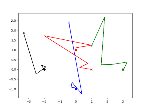
Here is a plot of the iterates as they converge to the roots.

Each color corresponds to a different root. Each starts at the initial guess marked with × and ends at the root marked with a circle.

[1] Bernhard Reinke, Dierk Schleicher and Michael Stoll. The Weierstrass–Durand–Kerner root finder is not generally convergent. Mathematics of Computation. Volume 92, Number 339.

Mercator and polar projections

This post is a more quantitative version of the previous post. Before I said that straight lines on a Mercator projection map correspond to loxodrome spirals on a sphere. This post will make that claim more explicit.

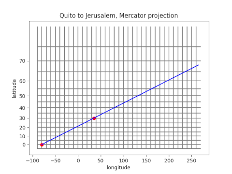
So suppose we plot a straight path from Quito to Jerusalem on a Mercator projection.

Quito to Jerusalem on a Mercator projection

The red dot in the lower left corner represents Quito and the next red dot represents Jerusalem.

Mercator projection leaves longitude λ unchanged, but latitude φ is transformed via

φ ↦ log( sec φ + tan φ )

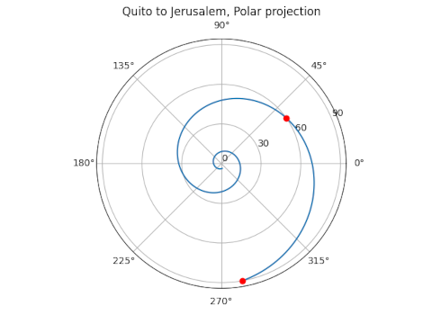
for reasons explained here. We can apply the inverse of the Mercator projection to put the path above on a globe, and when we do, it looks like the following.

Loxodrome path from Quito to Jerusalem on a polar plot

The path planned on a Mercator projection map when projected onto the globe becomes a logarithmic spiral in polar projection. The radial direction in the plot above shows the angle down from the North Pole rather than the angle up from the equator.

So if our flight of constant bearing keeps going rather than stopping at Jerusalem, it will spiral quickly toward the North Pole. It appears to stop at pole unless you look carefully. In theory the spiral keeps going and never actually reaches the pole. This is easy to see on the Mercator map because the North Pole is infinitely far away on the vertical axis.

Straight on a map or straight on a globe?

Straight lines on a globe are not straight on a map, and straight lines on a map are not straight on a globe.

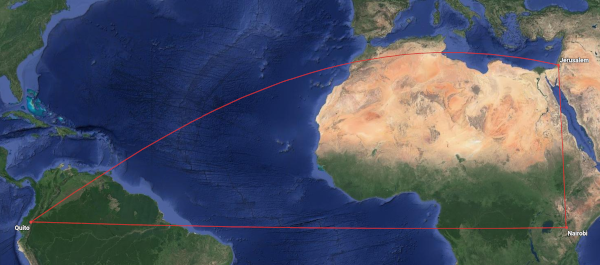
A straight line on a globe is an arc of a great circle, the shortest path between two points. When projected onto a map, a straight path looks curved. Here’s an image I made for a post back in August.

Quito to Nairobi to Jerusalem and back to Quito

The red lines form a spherical triangle with vertices at Quito, Nairobi, and Jerusalem. The leg from Quito to Nairobi is straight because it follows the equator. And the leg from Nairobi to Jerusalem is straight because it follows a meridian. But the leg from Quito to Jerusalem looks wrong.

If you were flying from Quito to Jerusalem and saw this flight plan, you might ask “Why aren’t we flying straight there, cutting across Africa rather than making a big arc around it? Are we trying to avoid flying over the Sahara?”

But the path from Quito to Jerusalem is straight, on a globe. It’s just not straight on the map. The map is not the territory.

Now let’s look at things from the opposite direction. What do straight lines on a map look like on a globe? By map I mean a Mercator projection. You could take a map and draw a straight line from Quito to Jerusalem, and it would cross every meridian at the same angle. A pilot could fly from Quito to Jerusalem along such a path without ever changing bearing. But the plane would have to turn continuously to stay on such a bearing, because this is not a straight line.

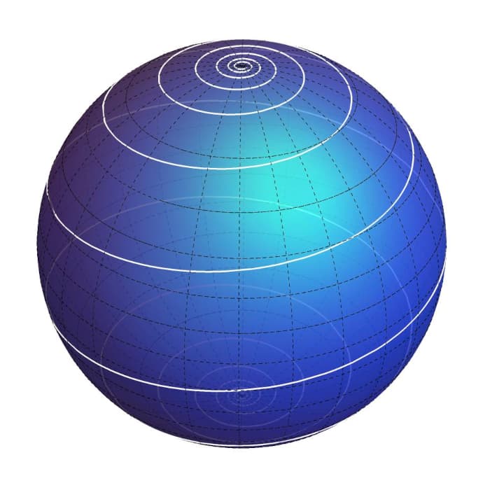
A straight line on a Mercator projection is a spiral on a globe, known as a loxodrome or a rhumb line. If a plane flew on a constant bearing from Quito but few over Jerusalem and kept going, it would spiral toward the North Pole. It would keep circling the earth, crossing the meridian through Jerusalem over and over, each time at a higher latitude. On a polar projection map, the plane’s course would be approximately a logarithmic spiral. The next post goes into this in more detail.

loxodrome spiral

I made the image above using the Mathematica code found here.

Although straight lines the globe are surprising on a map, straight lines on a map are even more surprising on a globe.

Related posts

Elliptic coordinates and Laplace’s equation

In rectangular coordinates, constant values of x are vertical lines and constant values of y are horizontal lines. In polar coordinates, constant values of r are circles and constant values of θ are lines from the origin.

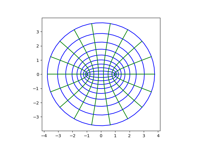
In elliptic coordinates, the position of a point is specified by two numbers, μ and ν. Constant values of μ are ellipses and constant values of ν are hyperbolas. (Elliptic coordinates could just as easily have been called hyperbolic coordinates, but in applications we’re usually more interested in the ellipses and so the conventional name makes sense.)

As with rectangular and polar coordinates, elliptic coordinates are orthogonal, i.e. holding each coordinate constant separately gives two curves that are perpendicular where they intersect.

Here’s a plot, with curves of constant μ in blue and curves of constant ν in green.

Graph paper for elliptic coordinates

The correspondence between rectangular and elliptic coordinates is given below.

x = a cosh μ cos ν
y = a sinh μ sin ν

The value of a can be chosen for convenience. More on that below.

Notice that elliptic coordinates area approximately polar coordinates when μ is large. This is because cosh(μ) approaches sinh(μ) as μ increases. For small values of μ elliptic coordinates are very different from polar coordinates.

The purpose of various coordinate systems is to adapt your coordinates to the structure of your problem. If you’re working with something that’s radially symmetric, polar coordinates are natural. And if you’re working with an ellipse, say you’re computing the electric field of an ellipse with uniform charge, then elliptic coordinates are natural. Ellipses can be described by one number, the value of μ.

Separation of variables

However, the real reason for specialized coordinate systems is solving partial differential equations. (Differential equations provided the motivation for a great deal of mathematics; this is practically an open secret.)

When you first see differential equations, the first, and possibly only, technique for solving PDEs you see is separation of variables. If you have PDE for a function of two variables u(x, y), you first assume u is the product of a function of x alone and a function of y alone:

u(x, y) = X(x) Y(y).

Then you stick this expression into your PDE and get independent ODEs for X and Y. Then sums of the solutions (i.e. Fourier series) solve your PDE.

Now, here’s the kicker. We could do the same thing in elliptic coordinates, starting from the assumption

u(μ, ν) = M(μ) N(ν)

and stick this into our PDE written in elliptic coordinates. The form of a PDE changes when you change coordinates. For example, see this post on the Laplacian in various coordinate systems. When you leave rectangular coordinates, the Laplacian is no longer simply the sum of the second partials with respect to each variable. However, separation of variables still works for Laplace’s equation using elliptic coordinates.

Separable coordinate systems get their name from the fact that the separation of variables trick works in that coordinate system. Not for all possible PDEs, but for common PDEs like Laplace’s equation. Elliptic coordinates are separable.

If you’re solving Laplace’s equation on an ellipse, say with a constant boundary condition, the form of the solution is going to be complicated in rectangular coordinates, but simpler in elliptic coordinates.

Confocal elliptic coordinates

The coordinate ellipses, curves with μ constant, are ellipses with foci at ±a; you can choose a so that a particular ellipse you’re interested has a particular μ value, such as 1. Since all these ellipses have the same foci, we say they’re confocal. But confocal elliptic coordinates are something slightly different.

Elliptic coordinates and confocal elliptic coordinates share the same coordinate curves, but they label them differently. Confocal elliptic coordinates (σ, τ) are related to (ordinary) elliptic coordinates via

σ = cosh μ
τ = cos ν

Laplace’s equation is still separable under this alternate coordinate system, but it looks different; the expression for the Laplacian changes because we’ve changed coordinates.

Related

Computing arccos

Suppose you take two numbers, a and b, and repeatedly take their arithmetic mean and their geometric mean. That is, suppose we set

a0 = a
b0 = b

then

a1 = (a0 + b0)/2
b1 = √(a0 b0)

and repeat this process, each new a becoming the arithmetic mean of the previous a and b, and each new b becoming the geometric mean of the previous a and b. The sequence of a‘s and b‘s converge to a common limit, unsurprisingly called the arithmetic-geometric mean of a and b, written AGM(a, b).

Gauss found that AGM(a, b) could be expressed as an elliptic integral K:

AGM(a, b) = π(a + b) / 4K((a − b)/(a + b)).

You might read that as saying “OK, if I ever need to compute the AGM, I can do it by calling a function that evaluates K.” That’s true, but in practice it’s backward! The sequence defining the AGM converges very quickly, and so it is used to compute K.

Because the AGM converges so quickly, you may wonder what else you might be able to compute using a variation on the AGM. Gauss knew you could compute inverse cosine by altering the AGM. This idea was later rediscovered and developed more thoroughly by C. W. Borchardt and is now known as Borchardt’s algorithm. This algorithm iterates the following.

a1 = (a0 + b0)/2
b1 = √(a1 b0)

It’s a small, slightly asymmetric variant of the AGM. Instead of taking the geometric mean of the previous a and b, you take the geometric mean of the new a and the previous b.

I am certain someone writing a program to compute the AGM has implemented Borchardt’s algorithm by mistake. It’s what you get when you update a and b sequentially rather than simultaneously. But if you want to compute arccos, it’s a feature, not a bug.

Borchardt’s algorithm computes arccos(a/b) as √(b² – a²) divided by the limit of his iteration. Here it is in Python.

    def arccos(a, b):
       "Compute the inverse cosine of a/b."
        assert(0 <= a < b) 
        L = (b**2 - a**2)**0.5 
        while abs(a - b) > 1e-15:
            a = 0.5*(a + b)
            b = (a*b)**0.5
        return L/a

We can compare our implementation of inverse cosine with the one in NumPy.

    import numpy as np

    a, b = 2, 3
    print( arccos(a, b) )
    print( np.arccos(a/b) )

Both agree to 15 figures as we’d hope.

A small variation on the function above can compute inverse hyperbolic cosine.

    def arccosh(a, b):
        "Compute the inverse hyperbolic cosine of a/b."
        assert(a > b > 0)
        L = (a**2 - b**2)**0.5
        while abs(a - b) > 1e-15:
            a = 0.5*(a + b)
            b = (a*b)**0.5
        return L/a

Again we can compare our implementation to the one in NumPy

    a, b = 7, 4
    print( arccosh(a, b) )
    print( np.arccosh(a/b) )

and again they agree to 15 figures.

In an earlier post I wrote about Bille Carlson’s work on elliptic integrals, finding a more symmetric basis for these integrals. A consequence of his work, and possibly a motivation for his work, was to be able to extend Borchardt’s algorithm.” He said in [1]

The advantage of using explicitly symmetric functions is illustrated by generalizing Borchardt’s iterative algorithm for computing an inverse cosine to an algorithm for computing an inverse elliptic cosine.

I doubt Borchardt’s algorithm is used to compute arccos except in special situations. Maybe it’s used for extended precision. If you had an extended precision library without an arccos function built in, you could implement your own as above.

The practical value of Borschardt’s algorithm today is more likely in evaluating elliptic integrals. It also alludes to a deep theoretical connection between AGM-like iterations and elliptic-like integrals.

Related posts

[1] B. C. Carlson. Hidden Symmetries of Special Function. SIAM Review , Jul., 1970, Vol. 12, No. 3 (Jul., 1970), pp. 332‐345

Three diagrams

This post will give examples of three similar diagrams that occur in three dissimilar areas: design of experiments, finite difference methods for PDEs, and numerical integration.

Central Composite Design (CCD)

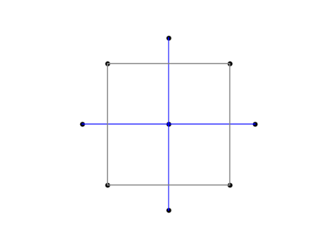
The most popular design for fitting a second-order response surface is the central composite design or CCD. When there are two factors being tested, the combinations of the two factors are chosen according to the following diagram, with the value at the center being used for several replications, say four.

CCD grid

The variables are coded so that the corners of the square have both coordinates equal to ±1. The points outside the square, the so-called axial points, have one coordinate equal to 0 and another equal to ±√2.

Finite difference method

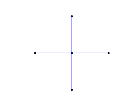
The star-like arrangement of points with the middle being weighted more heavily is reminiscent of the five-point finite difference template for the Laplacian. Notice that the center point is weighted by a factor of −4.

 h^2 \, \nabla^2 u(0,0) \approx u(h, 0) + u(0, h) + u(-h, 0) + u(0, -h) - 4u(0,0)

In the finite difference method, this pattern of grid points carries over to a pattern of matrix coefficients.

Integrating over a disk

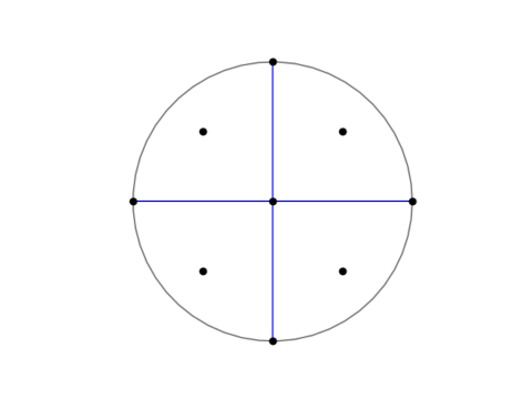
The CCD grid looks even more like a numerical integration pattern for a function f defined over a disk of radius h. See A&S equation 25.4.61.

\frac{1}{h^2} \int\!\int_D f(x, y)\, dx\,dy \approx \sum w_i\,f(x_i, y_i)

The center of the circle has weight w = 1/6. The four points on the circle are located at (±h, 0) and (0, ±h) and have weight w = 1/24. The remaining points are located at (±h/2, ±h/2) and have weight w = 1/6.

Related posts

Carlson’s elliptic integrals

Bille Carlson (1924-2013)

Although its a little fuzzy to say exactly which functions are “special” functions, these are generally functions that come up frequently in applications, that have numerous symmetries, and that satisfy many useful identities. The copious interconnections between special functions that are part of what makes them special also makes these functions hard to organize: everything is connected to everything else.

Bille Carlson did a great deal to simplify the study of special functions. With the benefit of decades of hindsight, Carlson discovered how several special functions should have been defined. I wrote a few weeks ago about how Carlson’s approach to Bessel functions eliminates unnecessary branch cuts. This post will look at how he simplified elliptic integrals.

The previous post looked at Legendre’s theorem showing that all elliptic integrals can be expressed in terms of three special functions—F, E, and Π— along with elementary functions. Carlson showed that Legendre’s three functions could be expressed in terms of two new functions. The advantage to Carlson’s approach is not that he reduced three functions down to two, but that his functions are symmetric. Hidden symmetries of elliptic integrals become obvious by definition.

Carlson’s elliptic functions

Carlson’s two basic functions are RF and RJ defined below.

\begin{align*} R_F(x,y,z) &= \tfrac{1}{2}\int_0^\infty \frac{dt}{\sqrt{(t+x)(t+y)(t+z)}} \\ R_J(x,y,z,p) &= \tfrac{3}{2}\int_0^\infty \frac{dt}{(t+p)\sqrt{(t+x)(t+y)(t+z)}} \end{align*}

These functions are obviously symmetric in x, y, and z.

In addition, Carlson defined three more functions for convenience. The functions RC and RD are simple variations on RF and RJ.

\begin{align*} R_C(x,y) &= R_F(x, y, y) \\ R_D(x,y,z) &= R_J(x, y, z, z) \end{align*}

Finally, his function RG is defined by

 R_G(x,y,z) = \tfrac{1}{4}\int_0^\infty \frac{t\left(\frac{x}{t+x} + \frac{y}{t+y} + \frac{z}{t + z} \right)}{\sqrt{(t+x)(t+y)(t+z)}}\, dt

The function RG can be expressed in terms of RF and RD as follows, but the form above makes its symmetry obvious.

2R_G(x, y, z) = z R_F(x, y, z) - \tfrac{1}{3} (x-z)(y-z) R_D(x, y, z) + \sqrt{\frac{xy}{z}}

See [1].

Legendre to Carlson

Legendre’s elliptic integrals of the first, second, and third kinds can be related to Carlson’s symmetric functions as follows.

\begin{align*} F(\phi,k) &=\sin\phi R_F\left(\cos^2\phi,1-k^2\sin^2\phi,1\right) \\ E(\phi,k) &=\sin\phi R_F\left(\cos^2\phi,1-k^2\sin^2\phi,1\right) \\ &\phantom{=}-\tfrac{1}{3}k^2\sin^3\phi R_D\left(\cos^2\phi,1-k^2\sin^2\phi,1\right) \\ \Pi(\phi,n,k) &=\sin\phi R_F\left(\cos^2\phi,1-k^2\sin^2\phi,1\right) \\ &\phantom{=}+\tfrac{1}{3}n\sin^3\phi R_J\left(\cos^2\phi,1-k^2\sin^2\phi,1,1-n\sin^2\phi\right) \end{align*}

The correspondence between Legendre’s functions and Carlson’s functions is fairly complex. You could think of Carlson’s functions as a change of coordinates that makes things simpler, like describing the motion of planets from the perspective of the sun rather than the perspective of the earth.

The elliptic integrals discussed in this post have been the “incomplete” elliptic integrals. The identities for the corresponding complete elliptic integrals follow by setting φ = π/2.

\begin{align*} K(k) &=R_F\left(0,1-k^2,1\right) \\ E(k) &=R_F\left(0,1-k^2,1\right)-\tfrac{1}{3}k^2 \,R_D\left(0,1-k^2,1\right) \\ \Pi(n,k) &=R_F\left(0,1-k^2,1\right)+\tfrac{1}{3}n \,R_J \left(0,1-k^2,1,1-n\right) \end{align*}

Software support

In Python, scipy.special has functions ellipr* to implement each of Carlson’s R* functions. That is, elliprc, elliprd, elliprf, elliprg, and elliprj implement RC, RD, RF, RG, and RJ respectively.

Similarly, Mathematica has functions CarlsonR*. That is, CarlsonRC, CarlsonRD, CarlsonRF, CarlsonRG, and CarlsonRJ implement RC, RD, RF, RG, and RJ respectively.

Related posts

[1] B. C. Carlson. Numerical Computation of Real or Complex Elliptic Integrals. Available on arXiv.

Kinds of elliptic integrals

Adrien-Marie Legendre caricature watercolor

There are three fundamental kinds of elliptic integrals, and these are prosaically but unhelpfully called elliptic integrals of the first kind, the second kind, and the third kind. These names sound odd to modern ears, but it’s no different than classical musicians naming symphonies Symphony No. 1, Symphony No. 2, etc.

This post covers the classical forms of elliptic integrals dating back to Adrien-Marie Legendre (1752–1833) and the next post will cover the modern formulation by Bille Carlson (1924–2013).

Comparing Legendre and Beethoven

This post will present Legendre’s classification theorem for elliptic integrals, but first let’s look at a few similarities between Legendre and Beethoven.

The image above is a caricature of Legendre, which is unfortunately the only image we have of him. But in this watercolor Legendre looks a little like Beethoven.

Legendre was studying elliptic integrals while Beethoven was writing symphonies—Legendre published his classification of elliptic integrals around a year after Beethoven finished his 9th symphony—and there was a common aesthetic in how they named things

A name like “Symphony No. 5 in C minor” isn’t that descriptive. If we know the difference between Beethoven’s Symphony No. 4 and Symphony No. 5, it’s because we’ve become familiar with each symphony; the names alone aren’t significant. It’s not as if Beethoven’s fourth symphony was written in 4/4 time and his fifth in 5/4 or anything like that.

But we just accept that that’s the way classical composers named things, and we should extend the same understanding to mathematics of the same era. Legendre named his functions analogously to the way Beethoven named his symphonies.

Elliptic integrals

Before we classify elliptic integrals, we should say what elliptic integrals are. These are functions of the form

f(x) = \int_0^x R(t, \sqrt{P(t)}) \, dt

where R is a rational function and P is a polynomial of degree three or four.

Classification

Legendre’s classification theorem says that any elliptic integral can be written as a linear combination of elementary functions and three special functions: F, E, and Π. These are the elliptic integrals of the first, second, and third kind, defined below. Said another way, you can evaluate elliptic integrals if you add just three advanced functions—FE, and Π— to the set of functions covered in a calculus class.

The elliptic integral of the second kind comes up in calculating the length of an elliptic arc, and the family of elliptic integrals take their name from this association. I think of E as mnemonic for “ellipse” and F as mnemonic for “first.” I don’t know whether this was the original motivation for the names. Legendre was French, and I doubt he would call a function F for “first” because the French word for “first” is première. Maybe an English speaker came up with the notation.

Elliptic integrals of the first kind describe the motion of a pendulum [1]. So you might think of F as pendulum functions. It would have been nice if these functions were denoted P rather than F; French speakers could think P stands for “première” and English speakers could think it stand for “pendulum.”

At least in my experience, elliptic integrals of the second kind come up most often, with elliptic integrals of the first kind a distant second, and elliptic integrals of the third kind are rare. I believe my experience is typical; many sources only discuss integrals of the first and second kind and leave out integrals of the third kind.

Definitions

Here are Legendre’s three basic elliptic integrals.

\begin{align*} F(\varphi; k) &= \int_0^\varphi \frac{d\theta}{\sqrt{1 - k^2 \sin^2\theta}} \\ E(\varphi; k) &= \int_0^\varphi \sqrt{1 - k^2 \sin^2\theta} \, d\theta \\ \Pi(n; \varphi, k) &= \int_0^\varphi \frac{d\theta}{(1 - n\sin^2\theta)\sqrt{1 - k^2 \sin^2\theta}} \\ \end{align*}

Elliptic integrals versus elliptic functions

Elliptic integrals are functions defined by integrals. They’re not the same as elliptic functions, though there’s a connection. It is often said that the inverse of an elliptic integral is an elliptic function. That’s not true without some qualification. What’s true is that the inverse of an elliptic integral of the first kind is an elliptic function.

Related posts

[1] The equation for pendulum motion that is first introduced to students makes the simplifying assumption that the displacement angle θ is so small that sin θ can be replaced with θ. In this case the motion is described by sines and cosines. But if you don’t make this assumption, then the differential equation for motion is nonlinear and its solution is an elliptic integral of the first kind.