Solving hard problems

We help companies solve hard problems in mathematics, statistics, and computing. Let’s explore how we might work together.

Broadcasting and functors

Posted on 9 March 2021 by John

In my previous post, I looked at the map Δ that takes a column vector to a diagonal matrix. I even drew a commutative diagram, which foreshadows a little category theory.

Suppose you have a function f of a real or complex variable. To an R programmer, if x is a vector, it’s obvious that f(x) means to apply f to every component of a vector. Python (NumPy) works the same way, and calls this broadcasting. To a mathematician, this looks odd. What does the logarithm of a vector, for example, even mean?

As in the previous post, we can use Δ to formalize things. We said that Δ has some nice properties, and in fact we will show it is a functor.

To have a functor, we have to have categories. (Historically, functors came first; categories were defined in order to define functors.) We will define C to be the category of column vectors and M the category of square matrices as before. Or rather, we should say the objects of C are column vectors and the objects of M are square matrices.

Categories need morphisms, functions between objects [1]. We define the morphisms on C to be analytic functions applied componentwise. So, for example, if

z = [1, 2, -3],

then

tan(z) = [tan(1), tan(2), tan(-3)].

The morphisms on M will be analytic functions on square matrices, not applied componentwise but applied by power series. That is, given an analytic function f, we define f of a square matrix X as the result of sticking the matrix X into the power series for f. For an example, see What is the cosine of a matrix?

We said that Δ is a functor. It takes column vectors and turns them into square matrices by putting their contents along the diagonal of a matrix. We gave the example in the previous post that [4, i, π] would be mapped to the matrix with these elements on the diagonal, i.e.

$\Delta: \begin{pmatrix} 4 \\ i \\ \pi \end{pmatrix} \mapsto \begin{pmatrix} 4 & 0 & 0\\ 0 & i & 0 \\ 0 & 0 & \pi \end{pmatrix}$

That says what Δ does on objects, but what does it do on morphisms? It takes an analytic function that was applied componentwise to column vectors, and turns it into a function that is applied via its power series to square matrices. That is, starting with a function

$f(z) = \sum_{n=0}^\infty a_nz^n$

we define the morphism f on C by

$f : \begin{pmatrix} z_1 \\ z_2 \\ \vdots \\ z_n \end{pmatrix} \mapsto \begin{pmatrix} f(z_1) \\ f(z_2) \\ \vdots \\ f(z_n) \end{pmatrix}$

and the morphism Δ f on M by

$\Delta f : Z \mapsto \sum_{n=0}^\infty a_n Z^n$

where Z is a square matrix.

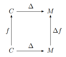
We can apply f to a column vector, and then apply Δ to turn the resulting vector into a diagonal matrix, or we could apply Δ to turn the vector into a diagonal matrix first, and then apply f (technically, Δf). That is, the follow diagram commutes:

$\begin{diagram} C & \rTo^{\Delta} & M \\ \uTo^{f} & & \uTo_{\Delta f} \\ C & \rTo^{\Delta} & M \end{diagram}$

Python example

Applying an analytic function to a diagonal matrix gives the same result as simply applying the function to the elements of the diagonal. But for more general square matrices, this is not the case. We will illustrate this with some Python code.

    import numpy as np
    from scipy.linalg import funm

    d = np.array([1, 2])
    D = np.diag(d)
    M = np.array([[1, np.pi], [2, 0]])

Now let’s look at some output.

    >>> np.sin(d)                     
    array([0.84147098, 0.90929743])   

    >>> np.sin(D)                     
    array([[0.84147098, 0.        ],  
           [0.        , 0.90929743]]) 

    >>> funm(D, np.sin)               
    array([[0.84147098, 0.        ],  
           [0.        , 0.90929743]])

So if we take the sine of d and turn the result into a matrix, we get the same thing as if we turn d into a matrix D and then take the sine of D, either componentwise or as an analytic function (with funm, function of a matrix).

Now let’s look at a general, non-diagonal matrix.

    >>> np.sin(M)
    array([[0.84147099, 0],
       [0.90929743, 0]])

    >>> funm(D, np.sin)
    array([[0.84147098, 0.        ],
           [0.        , 0.90929743]])

Note that the elements in the bottom row are in opposite positions in the two examples.

[1] OK, morphisms are not necessarily functions, but in practice they usually are.

Moving between vectors and diagonal matrices

Posted on 9 March 2021 by John

This is the first of two posts on moving between vectors and diagonal matrices. The next post is Broadcasting and functors.

Motivation

When I first saw the product of two vectors in R, I was confused. If x and y are vectors, what does x*y mean? An R programmer would say “You multiply components together, of course. What else could it mean?!”

But my first thought was “What kind of product do they mean? Inner product? Outer product? You can’t take the matrix product of two vectors.”

That was a long time ago. What brought this to mind today was a statistical paper I was reading that used the same symbol for a vector and a matrix. In context it wasn’t hard to figure out what the authors meant, but there was something implicit going on there that I will make explicit here.

Vectors and matrices

You can map a vector to a matrix by putting its contents along the diagonal of a diagonal matrix. That is, given a vector v of dimension n, create an n by n matrix V that is filled with zeros, except that

V_ii = v_i

for i = 1, 2, …, n. Let’s call this function Δ. In NumPy, Δ is implemented as the function diag. For example,

$\Delta: \begin{pmatrix} 4 \\ i \\ \pi \end{pmatrix} \mapsto \begin{pmatrix} 4 & 0 & 0\\ 0 & i & 0 \\ 0 & 0 & \pi \end{pmatrix}$

The statistics paper that I mentioned above used Δ implicitly, i.e. it denoted v and Δv with the same notation.

The function Δ has some nice properties.

The componentwise product two vectors is called the Hadamard product, denoted by a circle. You can first take the Hadamard product of two column vectors (of the same dimension) and then embed the result in a matrix using Δ, or you can first embed the two vectors into the world of matrices and take the product there. Either way you end up at the same place.

In other words, the following diagram commutes:

$\begin{diagram} C & \rTo^{\Delta} & M \\ \uTo^{\circ} & & \uTo_{\cdot} \\ C \times C & \rTo^{\Delta} & M \times M \end{diagram}$

Here C is the set of column vectors, and by C × C we mean pairs of column vectors of the same dimension. Similarly, M is the set of square matrices, and by M × M we mean pairs of square matrices of the same dimension. The circle on the left is Hadamard product. The dot on the right is ordinary matrix product [1].

The Δ on top is the Δ we’ve defined above. The Δ on bottom takes a pair of column vectors to a pair of matrices by operating on each element of the pair separately.

Although it would a little strange to do so, you could define Hadamard product this way. To take the Hadamard product of two vectors, take them over to the world of matrices, multiply the two matrices, and take that matrix back to the world of column vectors.

[1] Alternately, you could think of the product on the right as Hadamard product of matrices. For diagonal matrices, ordinary matrix product and Hadamard product coincide, though of course in general they are very different.

Adding tubes to knots

Posted on 7 March 2021 by John

Several months ago I wrote a blog post about Lissajous curves and knots that included the image below.

Lissajous knot

Here’s an improved version of the same knot.

Lissajous knot plotted in Mathematica with Tube function

The original image was like tying the knot in thread. The new image is like tying it in rope, which makes it easier to see. The key was to use Mathematica’s Tube function to thicken the curve and to see the crossings. I also removed the bounding box in the image.

This was the original code:

    x[t_] := Cos[3 t]
    y[t_] := Cos[4 t + Sqrt[2]]
    z[t_] := Cos[5 t + Sqrt[3]]
   
    ParametricPlot3D[{x[t], y[t], z[t]}, {t, 0, 2 Pi}]

The new code keeps the definitions of x, y, and z but creates a plot using Tube.

    
    Graphics3D[
        Tube[
             Table[{x[i], y[i], z[i]}, {i, 0, 2 Pi, 0.01}], 
             0.05
        ], 
        Boxed -> False
    ]

I went back and changed out the plots in my post Total curvature of a knot with plots similar to the one above.

A stiffening spring

Posted on 4 March 2021 by John

Imagine a spring with stiffness k₁ attached to a ceiling and a mass m₁ handing from the spring.

There’s a second spring attached to the first mass with stiffness k₂ and a mass m₂ handing from that.

mass spring system

The motion of the system is described by the pair of differential equations

$\begin{align*} m_1 x_1'' &= -k_1x_1 + k_2(x_2-x_1) \\ m_2 x_2'' &= -k_2(x_2 - x_1) \end{align*}$

If the second spring were infinitely stiff, the two masses would be joined with a rigid rod, and so the system would act like a single mass m₁ + m₂ hanging from the first spring. This motion would be described by the single differential equation

So it’s not surprising that as k₂ gets stiffer, the solution to the two-mass system converges to the solution to the system with a single combined mass. This is proven in [1].

However, what is missing from [1] is any visualization of how the solution to the two-mass system converges to that of the combined-mass system.

The plot below shows solutions for k₂ equal to 10, 100, and 1000, and finally the system to the combined-mass system, labeled k₂ = ∞. I used k₁ = 1, m₁ = 3, and m₂ = 5.

solution plots

The coupled-mass system has a high-frequency component due to the oscillation of the second mass relative to the first one.

The authors in [1] show that the amplitude of the high-frequency component decays as k₂ goes to infinity, though this is not apparent from the plots above. This is due to a limitation of the numerical method used to produce the plots.

Analytical solution

The numerical solution above raises two questions. First, how fast should the amplitude of high frequency component decay. Second, why did the numerical method apparently get the frequency of this component correct but the amplitude wrong?

The second question is more difficult and will have to wait for another post. The first question, however, we can settle fairly quickly.

The authors in [1] make the simplifying assumption that the two masses are equal to 1. They then define show that

$x_2(t) = \frac{d_1}{\alpha_2} \cos(\alpha_2 t) + \frac{d_2}{\alpha_2} \sin(\alpha_2 t) + \frac{d_3}{\alpha_4} \cos(\alpha_4 t) + \frac{d_4}{\alpha_4} \cos(\alpha_4 t)$

where the d‘s are constants that depend on initial conditions but not on the spring stiffnesses. and

$\begin{align*} a &= -(k_2 + 2k_2) \\ b &= \sqrt{k_1^2 + 4k_2^2} \\ \alpha_2 &= \sqrt{(b-a)/2} \\ \alpha_4 &= \sqrt{-(b+a)/2} \end{align*}$

α₄, the frequency of the low frequency component, approaches a finite limit as k₂ → ∞,

α₂, the frequency of the high frequency component, is approximately √(2k₂) for large k₂.

The amplitude of the high frequency component should be inversely proportional to its frequency.

tcgrep: grep rewritten in Perl

Posted on 3 March 2021 by John

In The Perl Cookbook, Tom Christiansen gives his rewrite of the Unix utility grep that he calls tcgrep. You don’t have to know Perl to use tcgrep, but you can send it Perl regular expressions.

Why not grep with PCRE?

You can get basically the same functionality as tcgrep by using grep with its PCRE option -P. Since tcgrep searches directories recursively, a more direct comparison would be

    grep -R -P

However, your version of grep might not support -P. And if it does, its Perl-compatible regular expressions might not be completely Perl-compatible. The man page for grep on my machine says

    -P, --perl-regexp
        Interpret the pattern as a Perl-compatible regular 
        expression (PCRE). This is experimental and grep -P 
        may warn of unimplemented features.

The one implementation of regular expressions guaranteed to be fully Perl-compatible is Perl.

If the version of grep on your system supports the -P option and is adequately Perl-compatible, it will run faster than tcgrep. But if you find yourself on a computer that has Perl but not a recent version of grep, you may find tcgrep handy.

Installation

tcgrep is included as part of the Unicode::Tussle Perl module; since tcgrep is a wrapper around Perl, it is as Unicode-compliant as Perl is. So you could install tcgrep (and several more utilities) with

    cpan Unicode::Tussle

This worked for me on Linux without any issues but the install failed on Windows.

I installed tcgrep on Windows by simply copying the source code. (I don’t recall now where I found the source code. I didn’t see it this morning when I searched for it, but I imagine I could have found it if I’d been more persistent.) I commented out the definition of %Compress to disable searching inside compressed files since this feature required Unix utilities not available on Windows.

Consistency

Another reason to use tcgrep is consistency. Perl is criticized for being inconsistent. The Camel book itself says

In general, Perl functions do exactly what you want—unless you want consistency.

But Perl’s inconsistencies are different, and in my opinion less annoying, than the inconsistencies of Unix tools.

Perl is inconsistent in the sense that functions behave differently in different contexts, such as a scalar context or a list context.

Unix utilities are inconsistent across platforms and across tools. For example, a tool like sed will have different features on different platforms, and it will not support the same regular expressions as another tool such as awk.

Perl was written to be a “portable distillation of Unix culture.” As inconsistent as Perl is, it’s more consistent that Unix.

Scaled Beta2 distribution

Posted on 3 March 2021 by John

I recently ran across a new probability distribution called the “Scaled Beta2” or “SBeta2” for short in [1].

For positive argument x and for positive parameters p, q, and b, its density is

$\frac{\Gamma(p+q)}{b\,\Gamma(p) \, \Gamma(q)}\, \frac{\left(\frac{x}{b}\right)^{p-1}}{\left(\left(\frac{x}{b}\right) + 1 \right)^{p+q}}$

This is a heavy-tailed distribution. For large x, the probability density is O(x^–q-1), the same as a Student-t distribution with q degrees of freedom.

The authors in [1] point out several ways this distribution can be useful in application. It can approximate a number of commonly-used prior distributions while offering advantages in terms of robustness and analytical tractability.

[1] The Scaled Beta2 Distribution as a Robust Prior for Scales. María-Eglée Pérez, Luis Raúl Pericchi, Isabel Cristina Ramírez. Available here.

Applications of (1-z)/(1+z)

Posted on 26 February 2021 by John

I keep running into the function

f(z) = (1-z)/(1+z).

The most recent examples include applications to radio antennas and mental calculation. More on these applications below.

Involutions

A convenient property of our function f is that it is its own inverse, i.e. f( f(x) ) = x. The technical term for this is that f is an involution.

The first examples of involutions you might see are the maps that take x to –x or 1/x, but or function shows that more complex functions can be involutions as well. It may be the simplest involution that isn’t obviously an involution.

By the way, f is still an involution if we extend it by defining f(-1) = ∞ and f(∞) = -1. More on that in the next section.

Möbius transformations

The function above is an example of a Möbius transformation, a function of the form

(az + b)/(cz + d).

These functions seem very simple, and on the surface they are, but they have a lot of interesting and useful properties.

If you define the image of the singularity at z = –d/c to be ∞ and define the image of ∞ to be a/c, then Möbius transformations are one-to-one mappings of the extended complex plane, the complex numbers plus a point at infinity, onto itself. In fancy language, the Möbius transformations are the holomorphic automorphisms of the Riemann sphere.

More on why the extended complex plane is called a sphere here.

One nice property of Möbius transformations is that they map circles and lines to circles and lines. That is, the image of a circle is either a circle or a line, and the image of a line is either a circle or a line. You can simplify this by saying Möbius transformations map circles to circles, with the understanding that a line is a circle with infinite radius.

Electrical engineering application

Back to our particular Möbius transformation, the function at the top of the post.

I’ve been reading about antennas, and in doing so I ran across the Smith chart. It’s essentially a plot of our function f. It comes up in the context of antennas, and electrical engineering more generally, because our function f maps reflection coefficients to normalized impedance. (I don’t actually understand that sentence yet but I’d like to.)

The Smith chart was introduced as a way of computing normalized impedance graphically. That’s not necessary anymore, but the chart is still used for visualization.

Smith chart

Image Wdwd, CC BY-SA 3.0, via Wikimedia Commons.

Mental calculation

It’s easy to see that

f(a/b) = (b–a)/(b+a)

and since f is an involution,

a/b = f( (b–a)/(b+a) ).

Also, a Taylor series argument shows that for small x,

f(x)ⁿ ≈ f(nx).

A terse article [1] bootstraps these two properties into a method for calculating roots. My explanation here is much longer than that of the article.

Suppose you want to mentally compute the 4th root of a/b. Multiply a/b by some number you can easily take the 4th root of until you get a number near 1. Then f of this number is small, and so the approximation above holds.

Bradbury gives the example of finding the 4th root of 15. We know the 4th root of 1/16 is 1/2, so we first try to find the 4th root of 15/16.

(15/16)^1/4 = f(1/31)^1/4 ≈ f(1/124) = 123/125

and so

15^1/4 ≈ 2 × 123/125

where the factor of 2 comes from the 4th root of 16. The approximation is correct to four decimal places.

Bradbury also gives the example of computing the cube root of 15. The first step is to multiply by the cube of some fraction in order to get a number near 1. He chooses (2/5)³ = 8/125, and so we start with

15 × 8/125 = 24/25.

Then our calculation is

(24/25)^1/3 = f(1/49)^1/3 ≈ f(1/147) = 73/74

and so

15^1/3 ≈ (5/2) × 73/74 = 365/148

which is correct to 5 decimal places.

Update: See applications of this transform to mentally compute logarithms.

[1] Extracting roots by mental methods. Robert John Bradbury, The Mathematical Gazette, Vol. 82, No. 493 (Mar., 1998), p. 76.

Saxophone ranges

Posted on 26 February 2021 by John

Saxophone quartet

I stumbled on a recording of a contrabass saxophone last night and wondered just how low it was [1], so I decided to write this post giving the ranges of each of the saxophones.

The four most common saxophones are baritone, tenor, alto, and soprano. These correspond to the instruments in the image above. There are saxophones below the baritone and above the soprano, but they’re rare.

Saxophones have roughly the same range as the human vocal parts with the corresponding names, as shown in the following table.

$\begin{center} \begin{tabular}{lllrr} \hline Part & Sax SPN & Human SPN & Sax Hz & Human Hz\\ \hline Soprano & $A \flat_3$ -- $E \flat_6$ & $C_4$ -- $C_6$ & 208--1245 & 262--1047\\ Alto & $D \flat_3$ -- $A \flat_5$ & $F_3$ -- $F_5$ & 139--831 & 175--698\\ Tenor & $A \flat_2$ -- $E \flat_5$ & $C_3$ -- $C_5$ & 104--622 & 131--523\\ Baritone & $D \flat_2$ -- $A \flat_4$ & $G_2$ -- $G_4$ & 69--415 & 98--392\\ Bass & $A \flat_1$ -- $E \flat_4$ & $E_2$ -- $E_4$ & 52--311 & 82--330\\ \hline \end{tabular} \end{center}$

SPN stands for scientific pitch notation, explained here. Hz stands for Hertz, vibrations per second.

The human ranges are convenient two-octave ranges. Of course different singers have different ranges. (Different saxophone players have different ranges too if you include the altissimo range.)

If you include the rare saxophones, the saxophone family has almost the same range as a piano. The lowest note on a subcontrabass saxophone is a half step lower than the lowest note on a piano, and the highest note on the sopranissimo saxophone is a few notes shy of the highest note on a piano.

$\begin{center} \begin{tabular}{llr} \hline Part & Sax SPN & Sax Hz\\ \hline Sopranissimo & $A \flat_4$ -- $E \flat_7$ & 416--2490\\ Sopranino & $D \flat_4$ -- $A \flat_6$ & 277--1662\\ Soprano & $A \flat_3$ -- $E \flat_6$ & 208--1245\\ Alto & $D \flat_3$ -- $A \flat_5$ & 139--831\\ Tenor & $A \flat_2$ -- $E \flat_5$ & 104--622\\ Baritone & $D \flat_2$ -- $A \flat_4$ & 69--415\\ Bass & $A \flat_1$ -- $E \flat_4$ & 52--311\\ Contrabass & $D \flat_1$ -- $A \flat_3$ & 35--208\\ Subcontrabass & $A \flat_0$ -- $E \flat_3$ & 26--156\\ \hline \end{tabular} \end{center}$

Update

My intent when I wrote this post was to add some visualization. One thought was to display the data above on a piano keyboard. That would be a nice illustration, but it would be a lot of work to create. Then it occurred to me that what putting things on a piano is really just a way of displaying the data on a log scale. So I plotted the frequency data on a log scale, which was much easier.

Saxophone and human voice ranges

Fraction comparison trick

Posted on 25 February 2021 by John

If you want to determine whether

a/b > c/d,

it is often enough to test whether

a+d > b+c.

Said another way a/b is usually greater than c/d when a+d is greater than b+c.

This sounds imprecise if not crazy. But it is easy to make precise and [1] shows that it is true.

Examples

Consider 4/11 vs 3/7. In this case 4 + 7 = 11 < 11 + 3 = 14, which suggests 4/11 < 3/7, which is correct.

But the rule of thumb can lead you astray. For example, suppose you want to compare 3/7 and 2/5. We have 3 + 5 = 8 < 7 + 2 = 9, but 3/7 > 2/5.

The claim isn’t that the rule always works; clearly it doesn’t. The claim is that it usually works, in a sense that will be made precise in the next section.

Rigorous statement

Let N be a large integer, and pick integers a, b, c, and d at random uniformly between 1 and N. Let

x = a/b – c/d

and

y = (a+d) – (b+c).

Then the probability x and y are both positive, or both negative, or both zero, approaches 11/12 as N goes to infinity.

Simulation

I won’t repeat the proof of the theorem above; see [1] for that. But I’ll give a simulation that illustrates the theorem.

    import numpy as np
    
    np.random.seed(20210225)
    
    N = 1_000_000
    numreps = 10_000
    
    count = 0
    for _ in range(numreps):
        (a, b, c, d) = np.random.randint(1, N+1, 4, dtype=np.int64)
        x = a*d - b*c
        y = (a+d) - (b+c)
        if np.sign(x) == np.sign(y):
            count += 1
    print(count/numreps)

This prints 0.9176, and 11/12 = 0.91666….

The random number generator randint defaults to 32-bit integers, but this could lead to overflow since 10⁶ × 10⁶ > 2³². So I used 64-bit integers.

Instead of computing a/b – c/d, I multiply by bd and compute ad – bc instead because this avoids any possible floating point issues.

In case you’re not familiar with the sign function, it returns 1 for positive numbers, 0 for 0, and -1 for negative numbers.

The code suggests a different statement of the theorem: if you generate two pairs of integers, their sums and their products are probably ordered the same way.

Psychology

This post has assumed that the numbers a, b, c, and d are all chosen uniformly at random. But the components of the fractions for which you have any doubt whether a/b is greater or less than c/d are not uniformly distributed. For example, consider 17/81 versus 64/38. Clearly the former is less than 1 and the latter is greater than 1.

It would be interesting to try to assess how often the rule of thumb presented here is correct in practice. You might try to come up with a model for the kinds of fractions people can’t compare instantly, such as proper fractions that have similar size.

[1] Kenzi Odani. A Rough-and-Ready Rule for Fractions. The Mathematical Gazette, Vol. 82, No. 493 (Mar., 1998), pp. 107-109

Normal probability fixed point

Posted on 24 February 2021 by John

Let Z be a standard normal random variable. Then there is a unique x such that

Pr(Z < x) = x.

That is, Φ has a unique fixed point where Φ is the CDF of a standard normal.

It’s easy to find the fixed point: start anywhere and iterate Φ.

Here’s a cobweb plot that shows how the iterates converge, starting with -2.

Cobweb plot for normal CDF

The black curve is a plot of Φ. The blue stairstep is a visualization of the iterates. The stairstep pattern comes from outputs turning into inputs. That is, vertical blue lines connect and input value x to its output value y, and the horizontal blue lines represent sliding a y value over to the dotted line y = x in order to turn it into the next x value.

y‘s become x‘s. The blue lines get short when we’re approaching the fixed point because now the outputs approximately equal the inputs.

Here’s a list of the first 10 iterates.

So it seems that after 10 iterations, we’ve converged to the fixed point in the first four decimal places.

Solving hard problems

Broadcasting and functors

Python example

Moving between vectors and diagonal matrices

Motivation

Vectors and matrices

Related posts

Adding tubes to knots

A stiffening spring

Analytical solution

More differential equation posts

tcgrep: grep rewritten in Perl

Why not grep with PCRE?

Installation

Consistency

Related posts

Scaled Beta2 distribution

Related posts

Applications of (1-z)/(1+z)

Involutions

Möbius transformations

Electrical engineering application

Mental calculation

Saxophone ranges

Update

More saxophone posts

Fraction comparison trick

Examples

Rigorous statement

Simulation

Psychology

Related posts

Normal probability fixed point