If three circles are all tangent to each other, you can find two more circles that are tangent to all three, and the equation for finding these new circles is remarkably elegant. This is Descartes’ theorem.
Two tangent circles
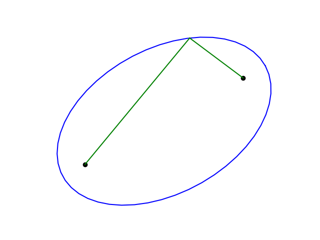
To illustrate Descartes’ theorem, we first need three mutually tangent circles. Drawing two mutually tangent circles is easy. We choose our coordinate system so that the first circle is centered at the origin
O1 = (x1, y1) = (0, 0)
and the center of the second circle is on the x-axis. If the two circles have radii r1 and r2, then the center of the second circle is at
O2 = (x2, y2) = (r1 + r2, 0).
I’ve assumed that the second circle is outside the first. You could have a tangent circle inside another circle, but to illustrate Descartes’ theorem we need circles that are externally tangent.
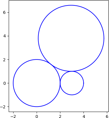
Three tangent circles
Now we pick the radius of the third circle to be r3. The center of this circle must belong to a circle of radius r1 + r3 centered at O1 and to a circle of radius r2 + r3 centered at O2. I went over finding the point(s) of intersection of two circles here.
For illustration I chose r1 = 2, r2 = 1, and r3 = 2.8. Using the code from the aforementioned post I found
(x3, y3) = (2.93333333 3.79941516)
Here’s a plot.
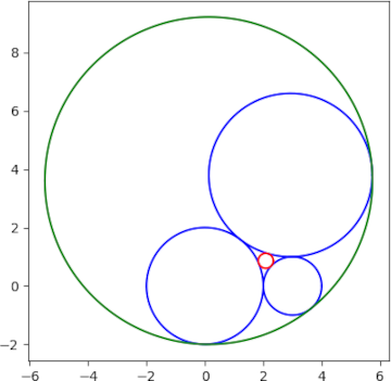
Four tangent circles
Now we’re in a position to state and illustrate Descartes’ theorem. The theorem is most easily stated in terms of signed curvatures.
The curvature of a circle of radius r is 1/r. Big circles have small curvature and small circles have big curvature.
For Descartes’ theorem we need to use signed curvatures, taking the sign to be positive if circles are externally tangent and negative if the circles are internally tangent. The signed curvatures of our three circles are positive, that is
ki = 1/ri
for i = 1, 2, and 3. But Descartes’ theorem will give us two circles, one between the three given circles and one surrounding them, corresponding to a positive and negative solution for k4.
Finding the radii
Now we can state Descartes’ theorem [1]:
(k1 + k2 + k3 + k4)² = 2(k1² + k2² + k3² + k4²)
This gives us a quadratic equation for k4 with two solutions:
k4 = k1 + k2 + k3 ±2(k1k2 + k2k3 + k1k3)½.
Finding the centers
Now we know the radii of our tangent circles, but not the centers. For this we view the circles as living in the complex plane with centers zi. Then the centers satisfy a theorem analogous to the one satisfied by the curvatures.
(k1z1 + k2z2 + k3z3 + k4z4)² = 2(k1²z1² + k2²z2² + k3²z3² + k4²z4²)
In other words, the curvature-center products satisfy the same equation as the curvatures.
I’m unclear on the history here, but I don’t believe Descartes had a formula for the centers of the circles. He certainly did not have the formula above using complex numbers [2].
Here’s a plot of the two circles guaranteed by Descartes’ theorem.
[1] The Soddy-Gossett theorem generalizes Descartes theorem to the case of n + 2 spheres in ℝn. The square of the sums of the curvatures equals n the sum of the curvatures squared.
[2] Jeffrey C. Lagarias, Colin L. Mallows, Allan R. Wilks. Beyond the Descartes circle theorem. https://arxiv.org/abs/math/0101066v1